Unsupervised Learning

This article is a summary note for CS3244 week 10 content.

Unsupervised machine learning is the machine learning task of inferring a function to describe hidden structure from “unlabeled” data (a classification or categorization is not included in the observations). Since the examples given to the learner are unlabeled, there is no evaluation of the accuracy of the structure that is output by the relevant algorithm.

1. Principal Components Analysis

What is Big data?

• Input data may have thousands or millions of dimensions!
• e.g., facial images, natural language text, stock market time series

Dimensionality reduction

• Advantages:
  • easier learning (due to fewer parameters)
  • faciliate visualization – hard to visualize more than 3D or 4D
  • discover “intrinsic dimensionality” of data
    • high dimensional data that is truly lower dimensional
• Example: Stock market data:
  • Presence of inherent stucture: Certain equities (like Transshipment stocks, Regional stocks) might change in a similar way
  • Use less information to get a good approximation
• Lower dimensional projections:
  • Rather than picking a subset of the features, we can create new features that are combinations of existing features.
  • 
• A review of linear projections:
  • Project a point into a (lower dimensional) spaces:
    1. Point: X = {x1,…,xn}
    2. Select a set of basis vectors: {v1,…,vk}
    3. We consider orthonormal bases: vi·vi = 1 and vi·vj = 0 if i ≠ j
    4. Select a center:
    • Take mean $\bar{x}$ of the dateset of all individual dimensions 5. Best coordinates in space (the transformed new coordinates in new space) defined by dot prudcts:
    • {z1,…,zk} where $z_{i} = (x-\bar(x))v_{k}$
    • Best = minimum squared error
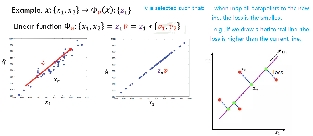
      PCA is a Projection from d-dimensional data into k-dimensional space while preserving information. We want to compute projection v with minimum reconstruction error: $\underset{z,v} \min \sum (x_{i}-z_{i}v)^{2}$
• v is choosed to minimize residual variance
• v is thus also the direction of maximum variance
• $z_{i}v$: the new $x’_{i}$ after projection

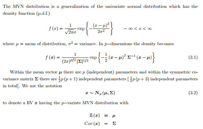
Recall if X follows Gaussian Distribution:

• The Mahalanobis distance $\Delta = \sqrt{(x-\mu)^{T}\Sigma^{-1}(x-\mu)}$, which represents the distance of the test point x from the mean μ
• $\Sigma$ is the covariance matrix $\Sigma = E[(X-\mu)(X-\mu)^{T}]$

Basic PCA Algorithm:

1. Start from d x N data matrix X
2. Re-center: subtract μ from each row of X ⇒ $X_{c} = X - \bar{X}$
3. (Typically) scale each dimension by its variance
   • To decorrelate the magnitude of variable
4. Compute covariance matrix: $\Sigma = \frac{1}{N} X_{c}^{T}X_{c}$
5. Find eigenvectors and eigenvalues of $\Sigma$
6. Compute K eigenvectors (Principal components) with highest eigenvalues

Method 2 and 3 refers to mean normalization (ensure every feature has zero mean) and optionally feature scaling.

For method 5 and 6, since we need to find the top k eigenvalues, we have 2 ways of doing this:

• Eigenvalue decomposition: $\Sigma = V\Lambda V^{T}$
  • $\lambda$ is the diagonal matrix of eigenvalues of the covarance $\Sigma$, usually in decreasing order ($\lambda_{1} > \lambda_{2} > …$)
  • V will the the matrix of eigenvectors corresponding to eigenvalues in $\Lambda$
  • To get top k eigenvectors, just take the first k columns of V
  • The new dataset will be V[:k] · $X_{c}$

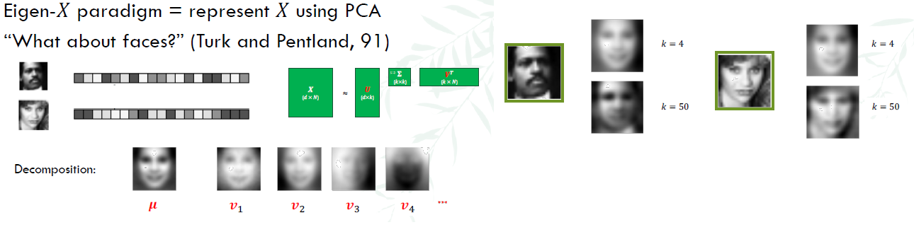
2. SVD and Eigenfaces

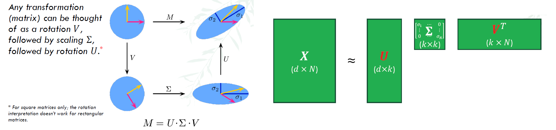
The singular value decomposition (SVD) factorizes a linear operator A : $R^{n}$ → $R^{m}$ into three simpler linear operators.

• $X = U\Sigma V^{T}$
  • U: m x r orthonomal matrix spanning X’s column space. Each row correponds to a datapoint –> coordinates of $x_{i}$ in eigenspace
  • $\Sigma$: r x r singular value matrix, a diagonal matrix with each entry $\sigma_{i}$ (Note that $\sigma_{i}(X) = \sqrt{\lambda_{i}(X^{T}X)}$ , λ is eigenvalue)
  • $V$: n x r orthonormal matrix spanning A’s row space

PCA using SVD Algorithm:

1. Start from d x N data matrix X
2. Re-center: subtract μ from each row of X ⇒ $X_{c} = X - \bar{X}$
3. (Typically) scale each dimension by its variance
   • To decorrelate the magnitude of variable
4. Compute covariance matrix: $\Sigma = \frac{1}{N} X_{c}^{T}X_{c}$

For method 5 and 6, since we need to find the top k eigenvalues, we have 2 ways of doing this:

• Singular Value Decomposition: $\Sigma = USV^{T}$
  • Take the first k vectors/columns of U (=$U_{reduced}$)
  • Z = $U_{reduced}^{T}x$ for $x \in X_{c}$
  • In this case, U = V, rows of $V^{T}$ are the eigenvectors of $X^{T}X = \Sigma$,too
  • Give the same eigenvectors as eigenvalue decomposition in this case, just that SVD is more numerically stable.

Eigenfaces

3. Clustering with K-means

A cluster is a collection of points S. A k-clustering is a partition of the data into k clusters S1,…Sk, where $\cup_{j=1}^{k} S_{j} = D$

• Each cluster has a center $\mu_{j}$
• Hard clustering assigns each point into exactly one cluster: $S_{i} \cap S_{j} = \emptyset$ for i ≠ j
• Points in a cluster should be similar (close to each other and the center)
• Error in cluster j: $E_{j} = \sum\limits_{x_{n}\in S_{j}} || x_{n}-\mu_{j}||_{2}^{2}$ (2-norm distance)
• Try to get class with $\min E_{in} = \sum\limits_{j=1}^{k} E_{j}$, however, this is not convex.

K means Algorithm

1. Choose k centers randomly (k is the number of classes you want to have)
2. Assign the K points to clusters, if the point is closest to center i, then this point is assigned to cluster i
3. Based on the points in each cluster, calculate new center for each cluster.
4. Repeat 2-3 until convergence

for k = 1 to K:
    mu[k] = some random location

while not converged:
    for n = 1 to N:
        y[n] = argmin_k ||mu[k] - x[n]||
    for k = 1 to K;
        mu[k] = (1 / n) * sum(x[n] for all n)
    # loop break when convergence

return y

• complexity: O(kN), k clusters and N points

Proof of Convergence

Only step 2 and 3 change values of μ and y. We can show that both can only decrease $E_{in}$

• $E_{in} \geq 0$ starts with some value after initialization
• As y is discrete, there can only be a finite number of steps, if each step can decrease $E_{in}$.
• Step 2: each time $|| x_{n}-\mu_{new}|| \leq || x_{n}-\mu_{old}||$ because you only reassign the point to new center if the point is closer to that new center
• Step 3: $\mu_{k}$ is calculated by mean of the points, which minimizes MSE (mean squared error)

Initialization

How to randomly select the means?

1. Furthest-first heuristic: after picking first point at random, pick all remaining k-1 centers to be as far as possible from all previously selected centers, i.e.:
   • $m = \text{arg}\underset{m}{\max} \,\underset{k’< k}{\min} || x_{m}-\mu_{k’}||$. Then set $\mu_{k} = x_{m}$
   • Deterministic after the first point selection.
2. K-means ++: When selecting $\mu_{k}$, choose point at random, but in probability proportional to squared distance (Add more randomness)
   • The following code can be summarized in 3 steps: compute distances, make probability distribution and pick example
   • for k = 2 to K:
     $\,d_{n} = \underset{k’< k}{\min} || x_{n}-\mu_{k’}||^{2}$, for all n
     $\, p = \frac{1}{\sum\limits_{n}\, n_{d}} d$
     $\, m = $ random sample from p
     $\, \mu_{k} = x_{m}$

Choosing K

How many clusters should I have in total? Should I add another cluster?

We can try different k, looking at the change in the average distance to centroid as k increases. However, using $E_{in}$ as a fitness measure is not good because it will always prefer:

1. Only 1 cluster for all points
2. The same number of cluster that I’m using now, K
3. n clusters for n points, each point in each cluster.
4. As k increases, it becomes a elbow shape, $E_{in}$ decreases slowly after some k.

Solution: Use regularization!

• Augment another term for optimization to ensure value of K is not overly complex.
  • Bayes Information Criterion (BIC): $\text{arg}\underset{k}{\min} E_{in}^{(k)} + k \log(d)$
  • Akaike Information Criterion (AIC): $\text{arg}\underset{k}{\min} E_{in}^{(k)} + 2kd$
• where d is the dimensionality of x
• model with better fit has lower AIC and BIC
• Penalize for dimension: 2-norm distance doesn’t work well in high dimensional space.

4. Gaussian Mixture Model (GMM)

GMMs can model data that comes from one of several known groups, where each group can be modeled by a Gaussian distribution. Fo e.g.

• The price of a paperback book is normally distributed with mean=$10.00 and standard deviation = $1.00 and the price of a hardback book is normally distributed with mean=$17.00 and standard deviation = $1.50
• Qn: is the price of a randomly choosen book normally distributed?
  • No, it’s bimodal.
• This model is a mixture of gaussians.
• Can we recover the component (individual Gaussian distributions) from the final distribution? That’s exactly what the EM algorithm (family) does.

Main idea: Clusters are modeled as Gaussians (not just by their mean like k-mean) with parameters (mean/covariance) unknown

• Expectation Maximization (EM) algorithm automatically discover all parameters for the K sources (clusters)

Mixture models in 1D

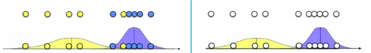
1. Given the figure in the left, we observe x1,…xn and knows that K=2 Gaussians with unknown $\mu, \sigma^{2}$. We can estimate for b(blue) cluster:
   • $\mu_{b} = \frac{x_{1}+…+x_{n_{b}}}{n_{b}}$ (mean of the group = the average of all datas in one group)
   • $\sigma^{2} = \frac{(x_{1}-\mu_{b})^{2}+…+ (x_{n_{b}} - \mu_{b})^{2}}{n_{b}}$ (variance calculated by using all datas in that group)
2. Given the figure in the right, we do not know the source, (which one is from yellow or blue)
   • if we know parameters of the gaussian ($\mu, \sigma^{2}$)
     • we can figure out which point is more likely to be in yellow or be in blue
   • Probability of blue given the data = $P(b|x_{i}) = \frac{P(x_{i}|b)P(b)}{P(x_{i}|b)P(b) + P(x_{i}| y)P(y)}$ (y stands for yellow)
   • $P(x_{i}|b)P(b) = \frac{1}{\sqrt{2\pi\sigma_{b}^{2}}}\exp(-\frac{(x_{i}-\mu_{b})^{2}}{2\sigma_{b}^{2}})$ is the p.d.f of Gaussian distribution
     

Gaussian mixture models with more than 1 dimension

Let’s say we have data with d dimensions(attributes), from k sources

• Each source c is a Gaussian
• iteratively estimate parameters:
  • prior: what percentage of instanes came from source c? $P(c) = \frac{1}{n}\sum\limits_{i=1}^{n} P(x|x_{i})$
  • mean: expected value of attribute j from source c. $\mu_{c,j} = \sum\limits_{i=1}^{n} (\frac{P(c|x_{i})}{nP(c)})x_{i,j}$
  • covariance: how correlated are attributes j and k in source c? $(\Sigma_{c}){j,k} = \sum\limits{i=1}^{n} (\frac{P(c|x_{i})}{nP(c)})(x_{i,j} - \mu_{c,j})(x_{i,k} - \mu_{c,k})$
  • based on: our guess of the source for each instance $P(c|x_{i}) = \frac{P(x_{i}|c)P(c)}{\sum\limits_{c’=1}^{k} P(x_{i}|c’)P(c’)}$

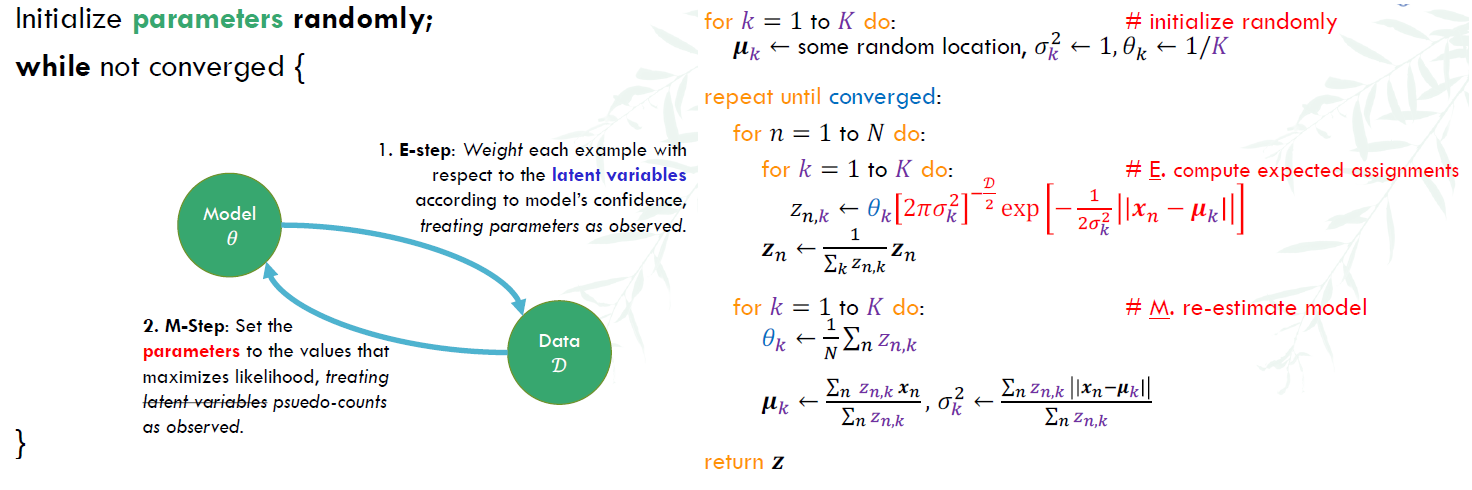
5. Expectation Maximization

Main idea of EM algorithm

1. start with K randomly placed Gaussians
2. For each point, assign it to the gaussian distribution which it is most likely to be from
3. Use the points of the same gaussian distribution, re-calculate mean and variance

How to pick K?

Properties of EM

EM is a local optimization function, but often the likelihood function is not convex. We’ll need to run EM several times with different random initializations and pick the parameters that yield the highest likelihood.

EM by other names

• Forward Backward: Use EM for estimating latent labels on sequential models (HMM: Hidden Markov Model) Inside Outside: Use EM for tree-like structures (like PCFGs: probabilistic context-free grammars)

Variants of EM

1. Generalized EM: Replace the M-Step by a single gradient-step that improves the likelihood
   • instead of increase to the maximum extend, we can increase slightly each time. Used when the maximization is difficult
2. Monte Carlo EM: Approximate the E-Step by sampling (instead of just assigning/estimation)
   • In complicated models for high-dimensional data, it is common to encounter an intractable integral in the E-step. The Monte Carlo EM algorithm works around this difficulty by maximizing instead a Monte Carlo approximation to the appropriate conditional expectation.
3. Sparse EM: Keep an “active list” of points (updated occasionally) from which we estimate the expected counts in the E-Step (only look at these points instead of the whole dataset)
   • Advantageous when the unobserved variable Y can take on many possible values, but only a small set of ‘plausible’ values have non-negligible probability.
4. Incremental EM / Stepwise EM: If standard EM is described as a batch algorithm, these are the online equivalent.
   • • It can converge to the vicinity of the correct answer more rapidly
   • Incremental EM increases L monotonically after each update by virtue of doing coordinate-wise ascent and thus is guaranteed to converge to a local optimum of both L and l
   • Stepwise EM might not increase either L or l after each update, but it is guaranteed to converge to a local optimum of `given suitable conditions on the stepsize discussed earlier.

References

1. Mixture Models