Decision Trees and Ensembling

Song Jiaming | 19 Nov 2017

This article is a summary note for CS3244 week 9 content. The note also includes some contents from Machine Learning Technique Course of National University of Taiwan.

1. Decision Trees

People often focus on just a few questions (dimensions) of an event.

Imperative programming control flow also embodies this. (if sth do sth, else do sth)

For example:

Parts of a tree:

Internal nodes, aka tests, a node tests exactly 1 component of x
A branch in the tree corresponds to a test result
- An attribute value or a range of attribute values
Each leaf node assigns:
- A class y ∈ {discrete classes} : (classification) decision tree
- Real value y ∈ R: regression tree

Decision Boundary: Tennis2

Important decisions are prefered to be at the top. 3 questions derived from above:

How do we pick a feature(branching critera) to split on?
How do we discretize continuous features?
How do we decide where to prune? (when to stop growing the tree, doesn’t work well in practice)

Decision Tree Learning

Path view

view the tree in the perspective of leafs, each leaf is in a path (from root to leaf)
- $G(x) = \sum\limits_{t=1}^{T}\, [[\text{is x on path t ?}]]\cdot g_{t}(x)$
- G(x): full-tree hypothesis
- $g_{t}(x)$: base hypothesis, leaf at the end of path t, a constant

Recursive view

view from the root, separate the tree into a few branches
- $G(X) = \sum\limits_{c=1}^{C}\, [[b(x) = c?]]\cdot G_{c}(x)$
- b(x): branching criteria
- $G_{c}(x_{0})$: sub-tree hypothesis at the c-th branch
Idea: (Recursively) choose most significant attribute as root of (sub) tree

A Basic Decision Tree Algorthm

Given dataset D = ${(x_{1},y_{1}),…,(x_{N},y_{N})}$

function DTL(D):
  if termination critera is met:
      return base hypothesis g_t(x)
  else:
      1) learn branching criteria b(x)
      2) split D to C parts: Dc = {(xn,yn): b(xn) = c}
      3) build subtree Gc = DLT(Dc) #build subtree based on branches
      4) return G(x)

More detailed pseudocode:

attributes: features
default: base hypothesis $g_{t}(x)$

CHOOSE_ATTRIBUTE: choose the best attribute out of a set

def DTL(D, attributes, default):
  if (D is empty): return default  # no example
  elif (all examples have the same classification): return the classification
  elif (attributes is empty): return MODE(D) # majority classification
  else:
  best = CHOOSE_ATTRIBUTE(attributes, D)
  tree = A new decision tree with best as the root
  for i in len(best):
      v = best[i]
      D[i] = {elements in examples with best = v}
      subtree = DTL(D[i], attributes= best, MODE(D))
      Add a branch to tree with label = v and subtree = subtree
  return tree

Classification and Regression Tree (CART) Algorithm

2 simple choices:
- C = 2 (binary tree)
- $g_{t}(x)$ is the constant that $\min E_{in}$
  - For Binary/Multiclass classification (0/1 errors): it is the majority of ${y_{n}}$
  - For Regression (squared error): it is the average of ${y_{n}}$
More simple choices:
- simple internal node for C = 2:{1,2}-output decision stump
- ‘easier’ sub-tree: branch by purifying
  - $b(x) = \underset{\text{decision stumps h(x)}}{\text{argmin}}\,\,\sum\limits_{c=1}^{2} |D_{c} \text{with h}| \cdot \text{impurity}(D_{c} \text{with h})$
- i.e. Bi-branching by purifying
Termination in CART: forced to terminate when:
- all $y_{n}$ the same: impurity = 0 $\implies g_{t}(x) = y_{n}$
- all $x_{n}$ the same: no decision stumps (fully-grown tree)

1.1 Choosing an attribute

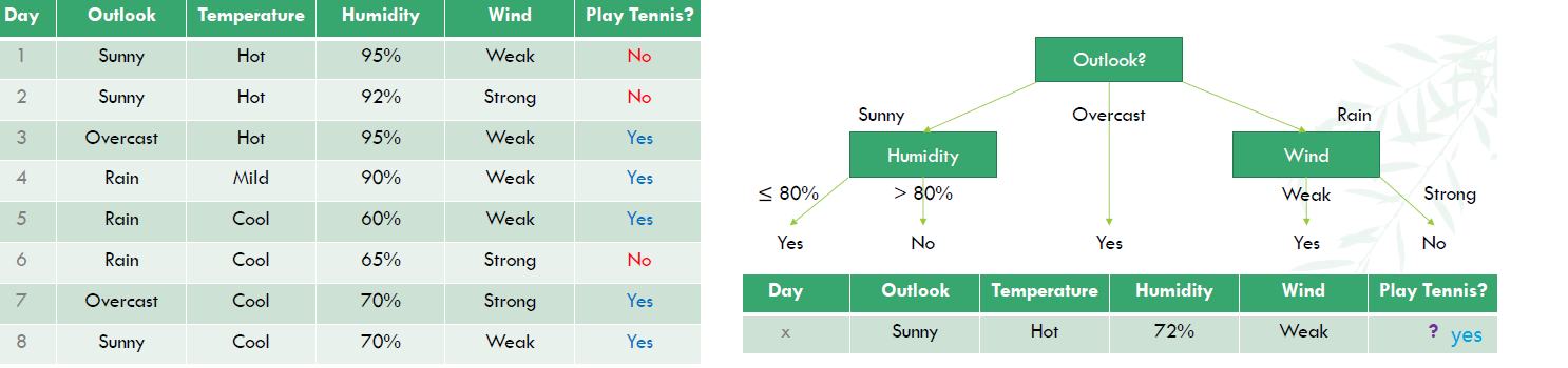
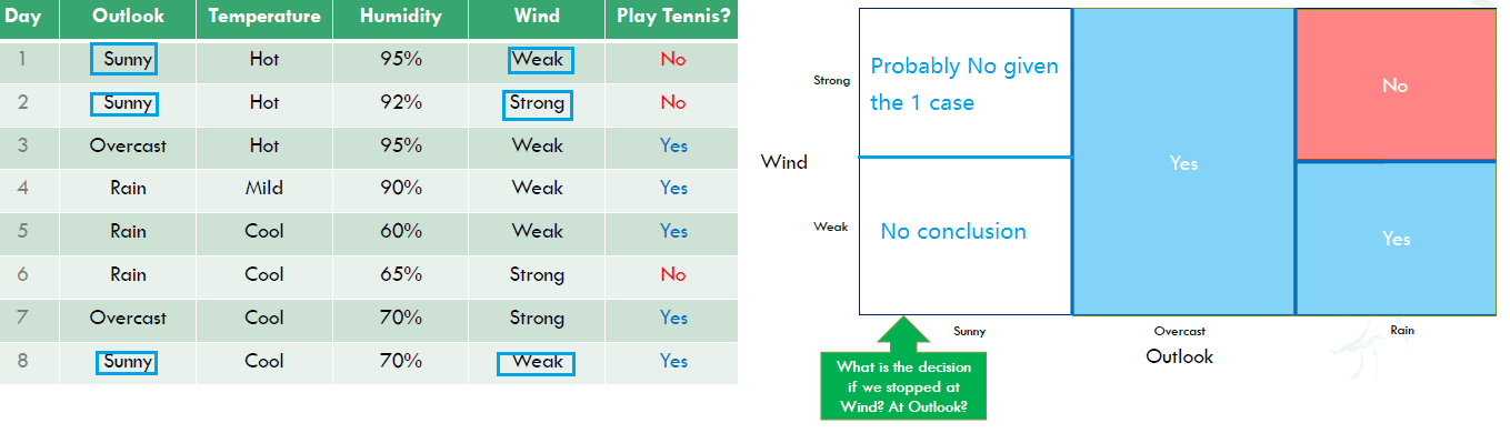
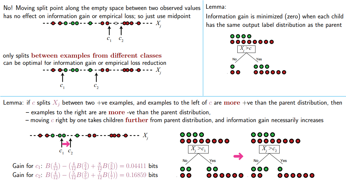
Overally, DTL algorithm maily refers to the algorithm to select the best attribute(feature) during the tree branching. The main idea is to select a good attribute that splits the training set into subsets that are as organised (pure) as possible. i.e. try to get “all positive” or “all negative” (purity) subsets

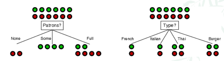
For the example below, patrons is a better choice, because of its purity of the subproblems. Attribute

Let’s cover 2 common ways to choose attributes in DTL.

Information gain
Gini impurity

Method 1: Information Gain

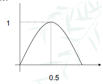
First we need to understand entropy, which is a common way to measure impurity. The higher the entropy the more the information content.

$H(X) = - \sum\limits_{x\in X} \, p(x)\, \log_{2}\,p(x)$
- p(x): probability of x happening
- Note that $\log_{b} x = \frac{\log_{a} x}{\log_{b} x}$
e.g. For a training set containing p positive examples and n negative examples, its entropy is:
- X contains events positive and negative
- P(positive) = $\frac{p}{p+n}$, P(negative) = $\frac{n}{p+n}$
- $H(\frac{p}{p+n},\frac{n}{p+n}) = -\frac{p}{p+n}\log(\frac{p}{p+n}) -\frac{n}{p+n}\log\frac{n}{p+n}$ (by definition)

Entropy	Curve
For P(positive) = $\frac{p}{p+n}$, the 2-class entropy is: 0 when $\frac{p}{p+n} = 0$ (all data belong to negative class, no information) 1 when $\frac{p}{p+n} = 0.5$ (50% data in either class, maximum impurity) 0 when $\frac{p}{p+n} = 1$ (all data belong to positive class, no information) monotonically increasing between 0 and 0.5 monotonically decreasing between 0.5 and 1

Information gain

We want to determine which attribute in a given set of training feature vectors is most useful for discriminating between the classes to be learned. Information gain tells us how important a given attribute is.

A chosen feature $x_{i}$ divides the example set S into subsets $S_{1},…S_{C}$ according to the labels C of $x_{i}$
The entropy of S then reduces to the entropy of each $S_{1},…S_{C}$:
- $\text{remainder}(S,x_{i})$ = $\sum\limits_{j=1}^{C_{i}} \, \frac{|S_{j}|}{|S|}\, H(S_{j})$ (Average entropy of the subsets)
H(S) is the entropy of the parent set $x_{i}$.
Information Gain (IG) is IG(S,$x_{i}$) = H(S) - remainder(S,$x_{i}$)
Choose the attribute with the largest IG
e.g. For the Patron graph above, there are 12 points with 6 green (p), 6 negative (n)
- $H(S) = H(\frac{6}{12},\frac{6}{12}) = 1$
- If we choose Patrons as the feature, it separates X into 3 sets with size [2, 4, 6], each subset has entropy [$H(0,1), H(1,0), H(\frac{2}{6},\frac{4}{6})$]= [0,0,0.91829] (remember to change to log2)
  - Remainder = $\sum\limits_{j=1}^{3} \, \frac{|S_{j}|}{|S|}\, H(S_{j}) = \frac{2}{12}\cdot 0 + \frac{4}{12}\cdot 0 + \frac{6}{12}\cdot 0.91829$ = 0.45915
  - IG(patrons) = H(S) - remainder = 1 - 0.45915 = 0.541 bits
- If we choose Type as the feature, it separates X into 4 sets with size [2, 2, 4, 4], each subset has entropy [$H(\frac{1}{2},\frac{1}{2}), H(\frac{1}{2},\frac{1}{2}), H(\frac{2}{4},\frac{2}{4}), H(\frac{2}{4},\frac{2}{4})$]= [1,1,1,1]
  - Remainder = $\sum\limits_{j=1}^{4} \, \frac{|S_{j}|}{|S|}\, H(S_{j}) = \frac{2}{12}\cdot 1 + \frac{2}{12}\cdot 1 + \frac{4}{12}\cdot 1+\frac{4}{12}\cdot 1$ = 1
  - IG(patrons) = H(S) - remainder = 1 - 1 = 0 bits
- Patrons has the highest IG and it will be chosen by DTL as the root

Method 2: Gini impurity

Used by the CART algorithm, Gini impurity is a measure of how often a randomly chosen element from the set would be incorrectly labeled if it was randomly labeled according to the distribution of labels in the subset. (i.e. $E_{in}$)

Gini impurity can be computed by $\sum\limits_{i=1}^{C} p_{i}\cdot (1-p_{i})$
- Total C different classes
- $p_{i}$: probability of a item in class i being chosen times
- $1-p_{i} = \sum_{k\not = i} p_{k}$: probability of mistakely choosing item in other classes k when item in class i should be chosen
It reaches its minimum (zero) when all cases in the node fall into a single target category.
Gini impurity (formally): $I_{G}(p) = \sum\limits_{i=1}^{C} p_{i}(1-p_{i}) = 1-\sum\limits_{i=1}^{C} p_{i}^{2}$

1.2 Branching on features

For numerical features, braching uses decision stump

b(x) = [[$x_{i}\leq \theta$]] + 1 with $\theta \in R$

Q2. How do discretize continuous features?
How can we choose among an infinite number of split points for a continuous feature $x_{j}$? i.e. there exists infinitely many possible split points c to define node test [$x_{j} > c$?]

For categorical features, branching uses the decision subset:

b(x) = [[$x_{i \in S}$]] + 1, with S ⊂ {1,2,…}
i.e. if we have 3 features, fever, pain, tired. We can decide [fever] goes to the left, and [pain, tired] go to the right, or other ways
CART handles categorical features easily.

Missing features by Surrogate Branch

Let’s say we have possible b(x) =[[weight $\leq$ 50kg]], but weight is missing during prediction.

What human do?
- Go get weight
- Use threshold on height instead. Because threshold on height may approximate threshold on weight
Surrogate branch:
- Maintain surrogate branch (substitues) $b_{1}(x),b_{2}(x),…\approx$ best branch b(x) during training
- allow missing feature for b(x) during prediction by using surrogate (but these surrogate b’(x) should behave similarly like b(x))
CART handles missing features easily

1.3. How do we decide where to prune?

Analyzing Decision Trees:

How expressive is the H of decision trees?

If no noise in y (fully-grown tree), one can always have $E_{in} = 0$ (all $x_{n}$ different)
It can express/shatter any point (Each x can be in a class y). ⇒ $d_{vc} = \infty$
However, it means that the trees have overfitting, high variance, because low-level trees built with small dataset (little information)

Solution

Use a regularizer $\Omega(G) = NoOfLeaves(G)$ to measure how many leaves at the end.

regularized decision tree: $\underset{\text{G}}{\text{argmin}}\, E_{in}(G) + \lambda \cdot \Omega(G)$ (aka. pruned decision tree)
However, we now cannot enumerate all possible G computationally
- $G^{(0)}$ = fully-grown tree
- $G^{(i)}$ = $\underset{\text{G}}{\text{argmin}}\, E_{in}(G)$ such that $G^{(i)}$ has 1-leaf removed from $G^{i-1}$
- i.e. Originally I have a $G^{(0)}$ with 10 leaves. First round, I remove each leaf one by one, and see when removing which leaf, the tree left has the lowest $E_{in}$, and that tree becomes $G^{(1)}$,…, continuously removing 1 leaf for each iteration, see which $G^{(i)}$ is the best regularized decision tree
How do we choose $\lambda$? Validation

2. Ensemble

Stock Market -Ensemble

T friends $g_{1},…g_{T}$ predict whether a stock will go up as g(x). We can:

Select the most trustworthy friend based on their usual performance Validation: $g(x) = g_{t^{\ast}}(x)$ with $t^{\ast}=\underset{t\in {1,…,T}}{\text{argmin}}\, E_{val}(g_{t}^{-})$
- Need one strong $g_{t}^{-}$ to guarantee small $E_{val}$
Let each friend have a vote:
- Uniform Vote: g(x) = sign($\sum\limits_{t=1}^{T} \, 1\cdot g_{y}(x)$)
Weight the friends’ predications non-uniformly
- Weighted Vote: g(x) = sign($\sum\limits_{t=1}^{T} \, \alpha_{t}\cdot g_{y}(x)$) where $\alpha_{t}\geq 0$
- i.e. trust some friends more, some friends less
- Method 1 and 2 are special case of this method:
  - To get method 1: let $\alpha_{t}$ = [[$smallest E_{val}(g_{t}^{-})$]]
  - To get method 2: let $\alpha_{t} = 1$
Combine the predictions conditionally
- Decision Trees! Base learner a decision stump
- $G(x) = \text{sign} (\sum\limits_{t=1}^{T}\, q_{t}(x)\cdot g_{t}(x))$ with $q_{t}(x)\leq 0$ is a condition
- Include method 3: setting $q_{t}(x) = \alpha_{t}$

Blending/Aggregation models: mix or combine hypothesis for better perfomance.

2.2 Uniform Blending (method 2)

If all $g_{t}$ the same (autocracy) ⇒ as good as 1 single $g_{t}$
If very different $g_{t}$ (diversity + democracy) ⇒ Majority can correct minority
Similar for multiclass: $G(x)=\underset{1\leq k \leq K}{\text{argmax}}\,\sum\limits_{t=1}^{T} [[g_{t}(x) = k]]$
How about regression?
- $G(x) = \frac{1}{T} \sum\limits_{t=1}^{T} g_{t}(x)$

Theoretical Analysis of Uniform Blending

Let’s fix a x, $G(x) = \frac{1}{T} \sum\limits_{t=1}^{T} g_{t}(x)$
G = mean($g_{t}$), mean(f) = f
\begin{align} \text{mean}([g_{t}(x) - f(x)]^{2}) &= \text{mean}(g_{t}^{2} - 2g_{t}f + f^{2}) \\ &= \text{mean}((g_{t}^{2}) - 2Gf + f^{2} \\ &= \text{mean}((g_{t}^{2}) -G^{2} + (G-f)^{2} \\ &= \text{mean}((g_{t}^{2}) -2G^{2} +G^{2} + (G-f)^{2} \\ &= \text{mean}(g_{t} -G)^{2} + (G-f)^{2}\end{align}
Finally, $\text{mean}(E_{out}(g_{t})) = \text{mean}(\varepsilon(g_{t} -G)^{2}) + E_{out}(G) \geq E_{out}(G)$ ⇒ average of base hypotheses better than the big hypothesis.
Main idea of uniform blending: reduced variance for more stable perfomance

2.2 Boostrap And Bagging

We have learnt aggregation only after obtaining the base hypothesis $g_{1},…g_{T}$. Can we learning, obtaining and combine g(x) at the same time?

Firstly, How do we obtain these $g$? Diversity.
- diveristy by different models: different g from different H
- diveristy by different parameters: learning rate = 0.001, 0.01,…,10
- diveristy by algorithm randomness: random PLA with different random seed
- diversity by data randomness: within-cross-validation hypotheses $g_{t}^{-}$
- Next, can we have diversity by data randomness without $g_{t}^{-}$? i.e. obtain different g using the same dataset.
  - Yes! Bootstrapping!

Bootstrapping is a statistical tool that re-samples from D to simulate $D_{t}$

From a finite data you have to simulate ‘new’ data
Bootstrap sample $\tilde{D}_{t}$: re-sample N examples from D uniformly with replacement, for data randomness.
- from the original dataset, randomly choosing N datapoints each time, with replacement)
- $\tilde{D}{t} \approx D{t}$

Bootstrap Aggregation (aka BAGging): A simple meta algorithm on top of base algorithm A

for t = 1,2,...,T:
  request size-N' data D'_t from bootstrapping
  obtain g_t by A(D'_t):
      G = uniform( {g_t} ) # uniform blending

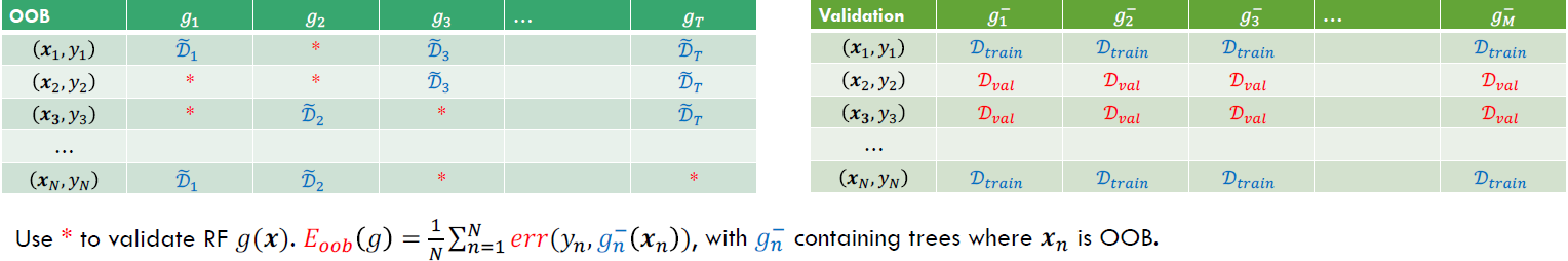
Out of Bag

The above method is also called the 0.632 bootstrap
- A particular training data has a probability of $1-\frac{1}{n}$ of not being picked (not used for obtained $g_{t}$, aka out-of-bag OOB examples for $g_{t}$)
- Thus its probability of ending up in the test data (not selected at all after N rounds of selection) is:
  - $(1- \frac{1}{n})^{n} \approx 2^{-1} = 0.368$ (OOB size per $g_{t}$)
- This means the training data will contain approximately 63.2% of the unique examples of original dataset, the rest are duplicate
- The final model G(x) = uniform(${g_{t}}$) has seen all the data points, for large N.
  - On average, an example will be in the majority of the bootstrap samples $\tilde{D}{t}$ (i.e. an example will be chosen at 63.2% as the bootstrap samples for training $g{t}$)
OOB versus Validation

Bagging reduces variance by averaging over many $g_{t}$ trained over different $\tilde{D}_{t}$, but has little effect on bias because it’s still working with the whole spectrum of H. Can we use more simplified H for learning in ensembles?

Boostrapping as a re-weighting process
$D = {(x_{1},y_{1}),…,(x_{4},y_{4})}$ via boostrap $\tilde{D}_{t} = {(x_{1},y_{1}),…,(x_{4},y_{4})}$ (choosed 1st sample, put it back, 2nd time also choosed 1st sample…)
set of $g_{T}$ is diverse by minimizing bootstrap weighted error

Weighted $E_{in}$ on D	$E_{in}$ on $\tilde{D}_{t}$
$E_{in}^{u}(h) = \frac{1}{4} \sum\limits_{n-1}^{4} \, u_{n}^{(t)} \cdot [[y_{n}\not = h(x_{n})]]$	$E_{in}^{0/1}(h) = \frac{1}{4} \sum\limits_{(x,y)\in \tilde{D}_{t}}^{4} \, [[y_{n}\not = h(x_{n})]]$
$(x_{1},y_{1}),u_{1} = 2$ $(x_{2},y_{2}),u_{2} = 1$ $(x_{3},y_{3}),u_{3} = 0$ $(x_{4},y_{4}),u_{4} = 1$	$(x_{1},y_{1})(x_{1},y_{1})$ $(x_{2},y_{2})$ $(x_{4},y_{4})$

2.3 Boosting

How can we improve upon bagging? Pay attention to the examples from the previous $g_{t-1}$ which we get right and which we get wrong:

increase the weight of examples we get wrong
decrease the weight of examples we get right

Boosting is an ensemble meta-algorithm to create strong learners from weak (slightly better than random) learners. It Reduces bias and variance, when weak learners are simple.

A choice as weak learner: Decision Stumps

$h_{s,i,\theta}(x) = s\cdot \text{sign}(x_{i}-\theta) = h(x;\theta_{i})$

Positive and negative rays on some features, 3 parameters: feature i, threshold θ, direction s
Visually, it is a line, axis-perpendicular planes in $R^{d}$
Efficient to optimize: O(d· log N) time
Allows efficient minimization of $E_{in}^{u}$, but can be too weak to work by itself.
Collect the outputs of the stumps into an ensemble:
- $h_{m}(x) = \sum\limits_{j=1}^{m}\alpha_{j} h(\textbf{x};\theta_{j})$

Adaptive Boosting (Adaboost)

We try to minimize the training loss $E_{in}$ corresponding to the ensemble $h_{m}(x) = h_{m-1}(\textbf{x})+\alpha_{m}h(\textbf{x};\theta_{m})$. Then we have:

$J(\alpha_{m},\theta_{m)} = \sum\limits_{t=1}^{t} W_{m-1}(t)\exp(-y_{t}\alpha_{m}h(x_{t};\theta_{m})$
Weighted ensemble $g(x_{n}) = \text{sign}(\sum\limits_{t=1}^{T} \alpha_{t}g_{t}(x_{n}))$
1. Set $W_{0}(t) = \frac{1}{n}$ for $t$ = 1,…,n.
2. At stage m, find a base learner $h(\textbf{x};\hat{\theta}_{m})$ that approximately minimizes $- \sum\limits_{t = 1}^{n} \hat{W}_{m-1}(t)y_{t}h(\textbf{x}_{t};\theta_{m}) = 2\epsilon_{m}-1$
3. Set $\hat{\alpha}_{m} = 0.5 \log(\frac{1-\hat{\epsilon_{m}}}{\epsilon_{m}})$
4. Update the weights on the training examples: $\hat{W}_{m}(t) = c_{m} \cdot \hat{W}_{m-1}(t) \exp(-y_{t}\hat{\alpha}_{m}h(\textbf{x}_{t};\hat{\theta}_{m}))$

The reassignining of weights (method 4):

$D_{t+1}(n) = \frac{D_{t}(n) \exp(-\alpha_{t}y_{n}g_{t}(x_{n}))}{Z_{t}}$
- $y_{n}g_{t}(x_{n}) > 0$ if prediction is correct ⇒ weight shrinks exponentially
- $y_{n}g_{t}(x_{n}) < 0$ if prediction is correct ⇒ weight grows exponentially
$Z_{t}$ is a normalizer to make weights for all training examples N sum to unity
$D_{\ast}$: can be thought as a probability distribution

Example

You have 6 training points (in some arbitrary space) (x1; x2; x3; x4; x5; x6) and 5 base classifier (weak learners) (h1; h2; h3; h4; h5). Each of these classifers makes the following misclassifications: e.g.

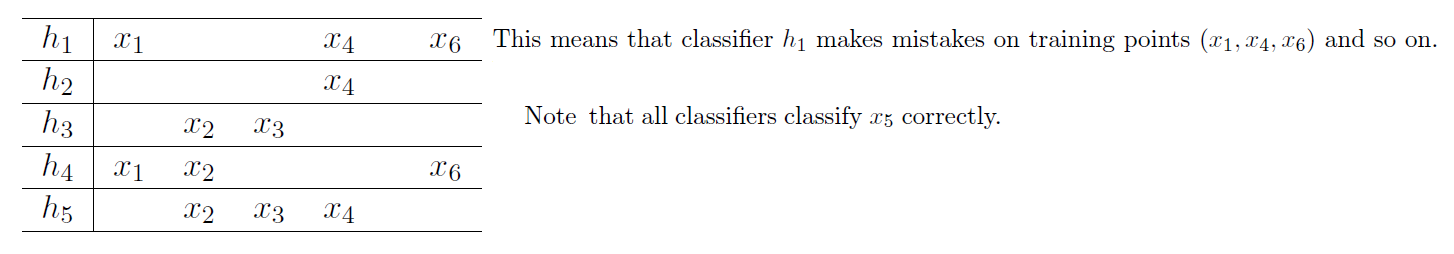
What are the initial weights $\tilde{W}_{0}(t)$ for t = 1,…,6?
- $\tilde{W}_{0}(t) = \frac{1}{6}$ for all t = 1,..6
Compute the weighted training error of each classifer based on weights $\tilde{W}_{0}(t)$
- Weighted training error for $h_{1} = \frac{3}{6}$, $h_{2} = \frac{1}{6}$, $h_{3} = \frac{2}{6}$, $h_{4} = \frac{3}{6}$, $h_{5} = \frac{3}{6}$. (proprotion of error to all points)
Which classifier would you choose in the first boosting round?
- $h_{2}$ as it has the smallest weighted training error
Compute the votes assigned to the first weak learner $\tilde{\alpha}_{1}$
- $\tilde{\alpha}_{1} = \frac{1}{2} \ln(\frac{1-\tilde{\epsilon}_{1}}{\tilde{\epsilon}_{1}}) = \frac{1}{2} \ln 5$
Compute the new set of weights $\tilde{W}_{1}(t)$ for t = 1,…, 6. Ensure that they sum to one.
- New weights for t = 1,2,3,5,6 (points that are classified correctly by $h_{2}$): $\tilde{W}_{1}(t) = c\cdot e^{-\frac{1}{2}\ln \,5} = \frac{c}{\sqrt{5}}$
- New weights for t = 4 (points that are classified wrongly by $h_{2}$): $\tilde{W}_{1}(t) = c\cdot e^{+\frac{1}{2}\ln \,5} =c\sqrt{5}$
- Thus $5 \cdot \frac{c}{\sqrt{5}} + c\sqrt{5} = 1$ ⇒ $c = \frac{1}{2\sqrt{5}}$ ⇒ substitute back
- $\tilde{W}_{1}(t) = \frac{1}{10}$ for t = 1,2,3,5,6, $\tilde{W}_{1}(t) = \frac{1}{2}$ for t = 4.
Compute the weighted training error of each classifer based on weights $\tilde{W}_{1}(t)$.
- $h_{1}$ made mistakes in $x_{1},x_{4}, x_{6}$, so its weighted traning error = $\frac{1}{10} + \frac{1}{2} + \frac{1}{10} = \frac{7}{10}$
- $h_{2}$ made mistakes in $x_{4}$ only, weighted training error = $\frac{1}{2}$
- Weighted training error for $h_{3}= \frac{2}{10}, h_{4}= \frac{3}{10},h_{5}= \frac{7}{10}$
Which classifer would you choose in the second boosting round?
- $h_{3}$ as its weighted training error is the smallest.
Suppose you continue the Adaboost procedure on the dataset (x1,…,x6) using the weak learners (h1,…, h5) a total of 2017 times. Which training point will have the lowest weight at the end of the 2017th round?
- x5 has the lowest weight since it is never misclassifed by any h.

2.4 Random Forests

Random forest = bagging + fully-grown CART decision tree

RandomForest(D):
    For t = 1,2,...,T:
        Sample D'_t via bootstrapping with D
        Obtain tree g_t by DTL(D'_t)
    return g(x) = uniform( {g_t} )

Highly parallel/efficient to learn
Inherits advantages of DTL
Lessens overfitting of fully-grown trees

In bagging, data randomness for diversity is made by randomly sample N examples from D. How about we randomly sample features instead?

randomly sample d’ features from x
often d’ « d, useful for large d, such as $d’ \equiv \sqrt{d}$
RF re-samples new feature subspaces for each tree b(x) in CART

Intuition behind random subspaces

Bagging can produce multiple $g_{t}$ that are correlated. The reason is that high IG features are likely to be the same over different bootstrapped samples.

When we sample d’ features, we attend DTL to just that subset of features, resulting in more diverse hypothesis $g_{t}$

Model Selection by OOB Error

$G_{m^{\ast}} = RF_{m^{\ast}}(D)$
$m^{\ast} = \underset{1\leq m\leq M}{\text{argmin}} \, E_{m}$
$E_{m} = E_{oob}(RF_{m}(D))$

$E_{oob}(G) = \frac{1}{N} \sum\limits_{n=1}^{N} err(y_{n}, G_{n}(x_{n})^{-}$
- $G_{n}(x_{n})^{-}$ contains trees which $x_{n}$ is OOB of this tree. For example, if $x_{n}$ is OOB of $g_{2}, g_{5}, g_{t}$, $G_{n}(x_{n})^{-}$ = average($g_{2}, g_{5}, g_{t}$)
Use $E_{oob}$ for self-validation of RF parameters such as d’’
no re-training needed

Feature Selection

For dataset x = (x1,…, xd), we want to remove:

redundant features: for e.g., keeping one of ‘age’ and ‘birthday’
irrelevant features: for e.g. education level for cancer prediction

Feature selection by importance

Idea: if possible to calculate importance(i) for i = 1,…, d, then can select top-d’ importance

Importance by linear model: $score=w^{T}x = \sum\limits_{i=1}^{d}w_{i}x_{i}$
- importance(i) = $|w_{i}|$, w learned from data
Importance by permutation test:
- idea: random test. If feature i needed, ‘random’ values of $x_{n,i}$ degrades performance
- which random values? bootstrap, permutation of {$x_{n,i}$}$_{n=1}^{N}$, $P(x_{i})$ approxmately remained
- importance(i) = performance(D) - performance($D^{(p)}$)
  - $D^{(p)}$ is dataset D with {$x_{n,i}$}, replaced by permuted {$x_{n,i}$}$_{n=1}^{N}$
  - Use OOB in RD to get performance. Now permutation test: importance(i) = $E_{oob}(G) - E_{oob}^{(p)}(G)$ (permutation during test, not permutation during training)