The VC dimension

Song Jiaming | 16 Nov 2017

This article is a summary note for CS3244 first half content of week 8. The lecture notes of this course used Caltech’s notes as reference.

1. Introduction to Hoeffding's Inequality

(related to the topic - Is Learning Feasible?)

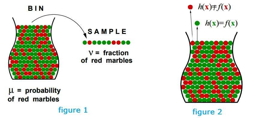
Consider a ‘bin’ with red and green marbles. (figure 1)
P[ piking a red marble] = µ (unknown)
P[ piking a green marble] = 1 − µ
We pick N marbles independently, these N marbles are our sample
- The fraction of red marbles in sample = v
(Possible) v cannot represent µ, sample can be mostly green while bin is mostly red
(Probable) but sample frequency v is likely close to bin frequency µ

In a big sample (large N), v is probably close to µ (within $\epsilon$). This is called Hoeffding’s Inequality:

$\mathbb{P}[ | v - \mu | > \epsilon ] \leq 2 e^{-2 \epsilon^{2} N}$
The probability of v is very different from µ is very small. i.e. “µ = v” is P.A.C (Probably Approximately Correct)
Observations from the inequality:
- Valid for all N and $\epsilon$
- Bound does not depend on µ
- Tradeoff between N, $\epsilon$ and the bound
- $v \approx \mu \implies \mu\approx v$

Connection to learning__(figure 2)

In Bin: the unknown is a number µ while in Learning: the unknown is a function f: X → Y
Each marble is a point x ∈ X
- when hypothesis predict x correctly (green): h(x) = f(x)
- when hypothesis predict x wrongly (red): h(x) $\not =$ f(x)
Bin analogy: probability distribution P on dataset X
- with assumption that, each x in X is generated by the distribution independently

bin

However, h is fixed, the color of the marbles are determined only by this h. So it is only verification of h, not learning.

We need to choose h from multiple h’s

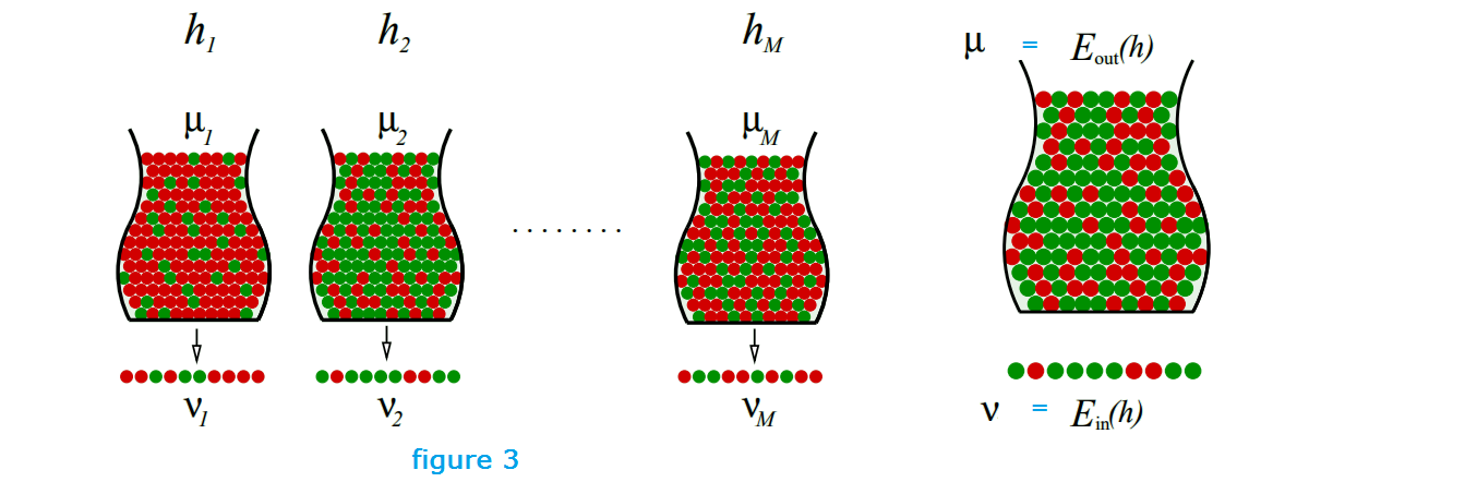
Notation for learning
Both µ and v depend on which hypothesis h.

v is ‘in sample’, denoted by $E_{in}(h)$, performance in samples you have seen
µ is ‘out of sample’, denoted by $E_{out}(h)$, performance in samples you have not seen

Now, the Hoeffding inequality becomes: $\mathbb{P}[ | E_{in}(h) - E_{out}(h) | > \epsilon ] \leq 2 e^{-2 \epsilon^{2} N}$

Hoeffding for multiple bins

However, Hoeffing inequality does not apply to multiple bins! Why?

If you toss a fair coin 10 times, P[10 heads] = 0.1%
If you toss 1000 fair coins 10 times each, P[some coin will get 10 heads] = 63% !
The 10 heads in 1000 coins case has no indication to the real problem

What can we do？We still want the difference between $E_{in}$ and $E_{out}$ to be small. Let’s start with left-hand side of Hoeffding inequality, \begin{align}\mathbb{P}[ | E_{in}(h) - E_{out}(h) | > \epsilon ] &\leq P[ | E_{in}(h_{1}) − E_{out}(h_{1})| > \epsilon \\ &\text{or } P[ | E_{in}(h_{2}) − E_{out}(h_{2})| > \epsilon \\ &\vdots \\ &\text{or } P[ | E_{in}(h_{M}) − E_{out}(h_{M})| > \epsilon \\ &\leq \sum\limits_{m=1}^{M} P[ | E_{in}(h_{m}) − E_{out}(h_{m})| > \epsilon \end{align}

The above is called the union bound, which is very loose. Equation (5) indicates the worst case
But since each of equation (1) to (4) corresponds to a single hypothesis, we can apply hoeffding equation to each of them: \begin{align}\mathbb{P}[ | E_{in}(h) - E_{out}(h) | > \epsilon ] &\leq \sum\limits_{m=1}^{M} P[ | E_{in}(h_{m}) − E_{out}(h_{m})| > \epsilon \\ &\leq \sum\limits_{m=1}^{M} 2 e^{-2 \epsilon^{2} N} \\ &= 2M e^{-2 \epsilon^{2} N}\end{align}

The approximation now depends on M (the size of hypothesis space H). If we have a very sophiscated model (M is large), the bound will not be tight and we loss the link between in-sample errors and out-of-sample errors

2. Growth function and Dichotomies

(related to the topic - Training vs. Testing)

In the previous section, we obtained an inequality with M, so where does this M come from?

The Bad events $B_{m}$ are $| E_{in}(h_{m}) - E_{out}(h_{m}) | > \epsilon$
i.e your in-sample performance does not track the out-of-sample perfomance
The probability of overall bad events is P[$B_{1}$ or $B_{2}$ or … or $B_{M}$] and we want the prbability of any of the bad events to be small.
- That’s because we want our algorithm to pick the hypothesis freely. If the probability of all bad events are small, then whatever hypothesis the algorithm pick will be ok
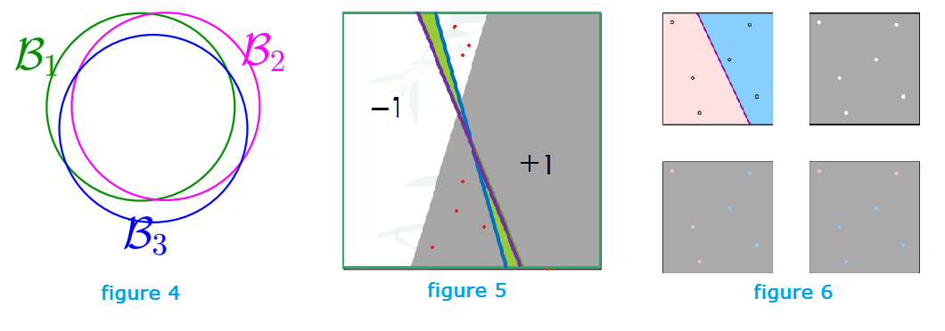
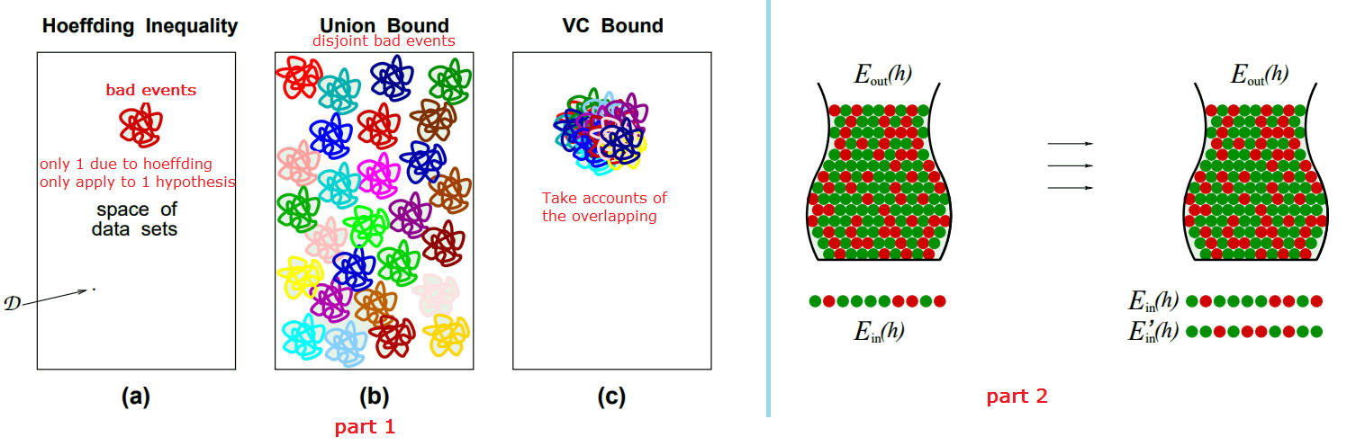
Bad events are overlapping (as shown in figure 4 below), we want to use union bound as if they are disjoint: P[$B_{1}$ or $B_{2}$ or … or $B_{M}$] $\leq P[B_{1}]+P[B_{2}]+…+P[B_{M}]$ (M terms, no overlap)

Can we improve on M?
Yes, in practice, bad event are extremely overlapping, so M is an overkill. Let’s look at figure 5 now. The blue line is the hypothesis,

$E_{out}$: the whole area of where the red dots lie in
$E_{in}$: just the red dots

Now, given a change of hypothesis from blue (h1) to purple (h2)

$\Delta E_{out}$: Change in +1 and -1 areas (green area)
$\Delta E_{in}$: Change in labels of data points

$| E_{in}(h_{1}) - E_{out}(h_{1}) | \approx | E_{in}(h_{2}) - E_{out}(h_{2}) |$ (They are overlapping, we can improve M)

Therefore, we want to define a quantity to replace M.

In figure 6, instead of the whole input space (like the 1st picture), we consider a finite set of input points and put them into the diagram (2nd picture), and count how many patterns of red or blue can we get using the hypothesis (like the 3rd and 4th picture)
We are going to call these patterns dichotomies.

Union Bound

Dichotomies

Given N data points and a hypothesis h: X → {-1, +1}, a dichotomy is $h:{x_{1},x_{2},…,x_{N} }$ → {-1,+1} (no. of patterns we can get from variation of h)

| H | can be infinite
| H($x_{1}$, $x_{2}$,…, $x_{N}$)| is at most $2^{N}$ (each point can be -1 or +1)

The growth function

The growth function counts the most dichotomies on any N points:

$m_{H}(N) = \underset{x_{1},…,x_{N}\in X}{\max} | H(x_{1}, x_{2},…, x_{N})|$
Out of any N points in the input space, the most dichotomies you can get
It satisfies: $m_{H}(N) \leq 2^{N}$

Examples: Applying $m_{H}(N)$ to perceptron

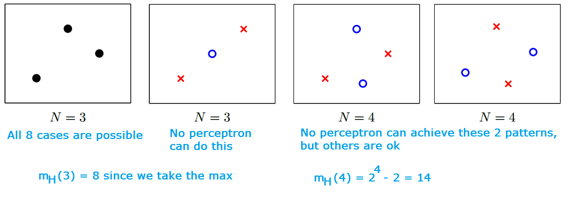
More Examples

So can we replace M with $m_{H}(N)$? Only if $m_{H}(N)$ is polynomial!

Break point

Definition: If no dataset of size k can be shattered by H, then k is a break point for H. i.e k is the point where you fail to give all possible dichotomies

$m_{H}(k) < 2^{k}$
For 2D perceptron, k = 4, as shown in the previous figure

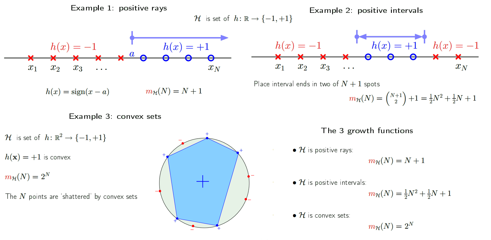
Back to the 3 examples:

Positive rays $m_{H}(N) = N+1$
- break point k = 2
Positive intervals $m_{H}(N) = \frac{1}{2}N^{2}+\frac{1}{2}N+1$
- break point k = 3
Convex sets $m_{H}(N) = 2^{N}$
- break point k = $\infty$ (no break point)

Therefore, if the hypothesis has no break point, it’s $m_{H}(N) = 2^{N}$, if there exists a break point, $m_{H}(N)$ is polynomial in N

3. Replace M with $m_{H}(N)$

(related to the topic - Theory of Generalization)

Proof $m_{H}(N)$ is polynomial

The proof can be done if we can show $m_{H}(N) \leq …\leq$ a Polynomial

Key Quantity B(N,k): Maximum no. of dichotomies on N points, with break point k.
Recursive bound Consider the following table (table 1):

Table

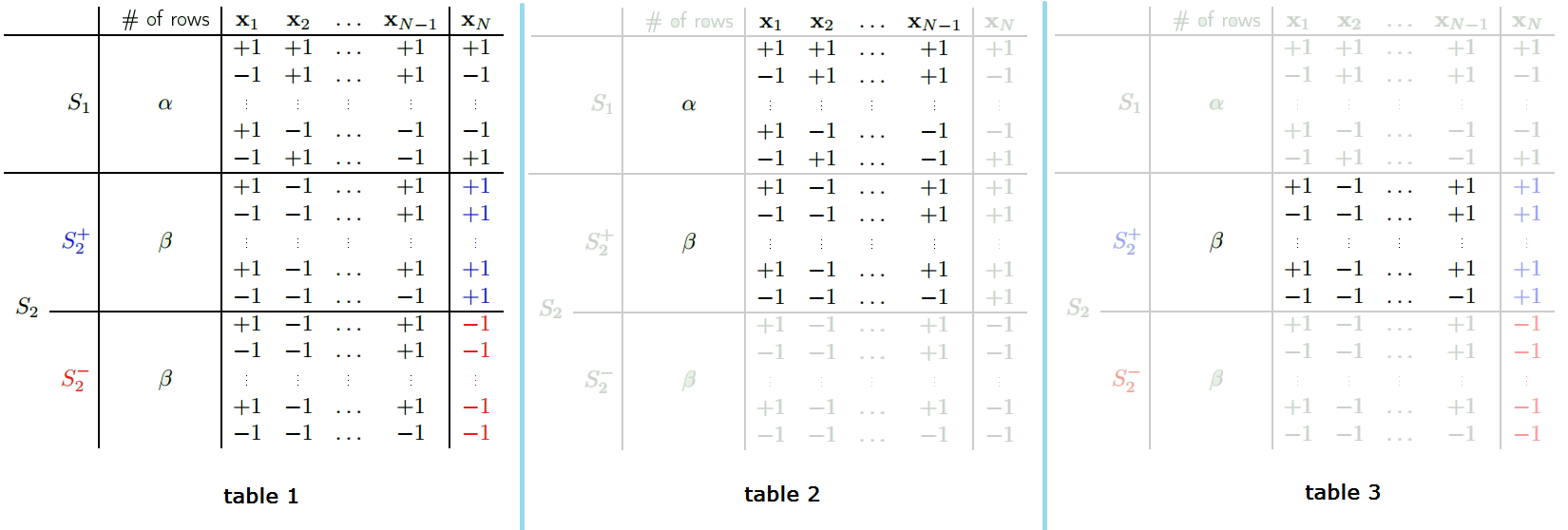
Since we want a recursion, we isolate the last element $x_{N}$

We separate all combinations into 2 groups:
- S1 includes rows with all different elements except the last elements:
  - e.g. [-1 +1 -1] and [+1 -1 -1] will be in S1, as only last element is the same. If there exists another [-1 +1 +1], then both [-1 +1 -1] and [-1 +1 +1] will be moved to S2
- S2 includes rows with the same elements except the last element. i.e. each pattern of $x_{1} … x_{N-1}$ happens twice in S2
  - e.g. [+1 -1 -1] and [+1 -1 +1] will be in S2, as they are identical except the last element
Then we separate S2 into 2 groups, one ends with +1, one ends with -1
We have, $B(N,k) = \alpha + 2\beta$

Then, only look at column $x_{1},…x_{N-1}$, are the rows different?

Yes in S1, because if there exists 2 rows identical, they would be in S2
In S2, since both pattern occurs twice with +1 and -1 extension, we take only 1 group, so now the rows in this 1 group are different
Now we have table 2. Therefore, $\alpha+\beta \leq B(N-1,k)$

Now, focus on $S2 = S2^{+} \cup S2^{-}$, still look at first N-1 columns only.

Since the 2 groups are identical, only look at $S2^{+}$ (table 3)
Claim it has at most k-1 break points. Because by extending back to the 2 copies and with the last column, the set can have all possible patterns for k points, which means B(N,k). But even for the whole set (with $\alpha$), the break point is k. So the $\beta$ rows couldn’t have k break points.
Now, $\beta \leq B(N-1,k-1)$

Together, $B(N,k) = \alpha + \beta + \beta$

$B(N,k) \leq B(N-1,k)+B(N-1,k-1)$
Theorem: $B(N,k) \leq \sum\limits_{i=0}^{k-1} \binom{N}{i}$
Can be proved using induction.
- Base step: when B(1,1), true.
- Induction step: \begin{align} \sum\limits_{i=0}^{k-1} \binom{N-1}{i} + \sum\limits_{i=0}^{k-2} \binom{N-1}{i} &= 1 + \sum\limits_{i=1}^{k-1} \binom{N-1}{i} + \sum\limits_{i=1}^{k-1} \binom{N-1}{i-1} \\ &= 1 + \sum\limits_{i=1}^{k-1} [\binom{N-1}{i} + \binom{N-1}{i-1}] \\ &= 1 + \sum\limits_{i=1}^{k-1} \binom{N}{i} \\ &= \sum\limits_{i=0}^{k-1} \binom{N}{i} \end{align}

For a given H, the break point k is fixed,

$m_{H}(N)\leq B(N,k) \leq \sum\limits_{i=0}^{k-1} \binom{N}{i}$ is polynomial! Because the maximum power is $N^{k-1}$ while k to any power is just a constant.

3 examples:

Positive rays (break point k =2)
- $m_{H}(N) = N+1 \leq N-1$
Positive intervals (break point k = 3)
- $m_{H}(N) = \frac{1}{2}N^{2}+\frac{1}{2}N+1 \leq \frac{1}{2}N^{2}+\frac{1}{2}N+1$
2D perceptrons(break point k = 4)
- $m_{H}(N) \leq \frac{1}{6}N^{3}+\frac{5}{6}N+1$

Proof $m_{H}(N)$ can replace M

We want $\mathbb{P}[ | E_{in}(h) - E_{out}(h) | > \epsilon ] \leq 2 (M\rightarrow m_{H}(N)) e^{-2 \epsilon^{2} N}$

Partial Proof:
- How $m_{H}(N)$ related to overlaps?
  - See part 1 of the figure below
- What to do about $E_{out}$
  - See part 2 of the figure below
  - Want to get rid of $E_{out}(h)$. Pick 2 samples: $E_{in}(h)$ and $E'_{in}(h)$
  - $E_{in}(h)$ and $E_{in}^{'}(h)$ track each other. (the same way as $E_{in}(h)$ and $E_{out}(h)$ track each other)
  - So now, instead of tracking $E_{out}$, we track 2 $E_{in}$, which is purely depends on the dichotomies. For 1 sample, we have N datapoints, now we have 2N datapoints

Canvas

Together:
- What we want is not quite: $\mathbb{P}[ | E_{in}(h) - E_{out}(h) | > \epsilon ] \leq 2 \, m_{H}(N)\, e^{-2 \epsilon^{2} N}$
- but rather $\mathbb{P}[ | E_{in}(h) - E_{out}(h) | > \epsilon ] \leq \bbox[pink]{4} \, m_{H}(\bbox[pink]{2}N)\, e^{-\bbox[pink]{\frac{1}{8}} \epsilon^{2} N}$
- The Vapnik-Chervonenkis Inequality
- Further more $\mathbb{P}[ | E_{in}(h) - E_{out}(h) | > \epsilon ] \leq 4 \, m_{H}(2N)\, e^{\frac{1}{8} \epsilon^{2} N} \leq 4 \, (2N)^{k-1}\, e^{\frac{1}{8} \epsilon^{2} N}$
  - if $m_{H}(N)$ breaks at k
  - N is large enough (a good dataset D) ⇒ probably generalized $E_{out} \approx E_{in}$
  - A picks a g with small $E_{in}$
  - ⇒ probably learned!

4. The VC Dimension

The VC dimension of a hypothesis set H, denoted by $d_{vc}(H)$ is:

the largest value of N (datapoints) for which $m_{H}(N) = 2^{N}$
“the most points H can shatter”
if a dataset have N points with $N \leq d_{vc}(H)$, ⇒ H can shatter these N points
if a number $k > d_{vc}(H)$, ⇒ k is the break point for H
$d_{vc} = k-1$ where k is the smallest break point

We know that $m_{H}(N) \leq \sum\limits_{i=0}^{k-1} \binom{N}{i}$

Now, $m_{H}(N) \leq \sum\limits_{i=0}^{d_{vc}} \binom{N}{i}$, where the maximum power is $N^{d_{vc}}$
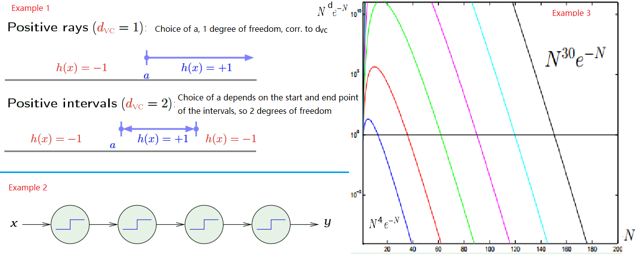
- Positive rays: cannot shatter 2 points ⇒ $d_{vc} = 1$
- 2D perceptrons: break point =4, $d_{vc} = 3$
- Convex sets: no break point, $d_{vc} = \infty$

VC dimension and Learning

$d_{vc}(H)$ is finite ⇒ g in H will generalize
Independent of Learning Algorithm
Indenpendent of Input Distribution
Independent of the Target Function

VC dimensions of perceptrons

For 2D perceptron, dimension d = 2, $d_{vc} = 3$

In general, $d_{vc} = d + 1$, d = dimension

To prove the equation, we prove in 2 directions $d_{vc} \leq d + 1$ and $d_{vc} \geq d + 1$

Show $d_{vc} \geq d + 1$
- Given a set of N = d+1 points in $\mathbb{R}^{d}$
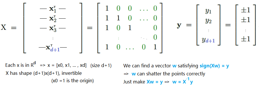
- Since we can find such w ⇒ we can shatter these d+1 points ⇒ $d_{vc} \geq d + 1$
Show $d_{vc} \leq d + 1$ ⇒ show that we cannot shatter any set of d+2 points. (Because the break point definition is that no dataset of size k can be shattered)
- Take any d+2 points, $x_{1},…,x_{d+1},x_{d+2}$
- There are more points (d+2) than dimension (x from $R^{d}$, has d+1 dimensions)
- So we must have one $x_{j}$ as the linear combinations of other points. i.e $x_{j} = \sum\limits_{i\not=j} a_{i}\,x_{i}$ and not all $a_{j}$ are 0.
- Consider the following dichotomy: the $x_{i}$ with $a_{i}\not = 0$ has $y_{i} = \text{sign}(a_{i})$. i.e, the points which are linearly dependent with $x_{j}$ has the same sign as its coefficient. And $x_{j}$ gets $y_{j} = -1$
- No w exists (no perceptron) to get the above dichotomy
  - $x_{j} = \sum\limits_{i\not=j} a_{i}\,x_{i} \implies w^{T}\,x_{j} = \sum\limits_{i\not=j} a_{i}\,w^{T}\,x_{i}$
  - If $y_{i} = \text{sign}(w^{T}\,x_{i}) = \text{sign}(a_{i})$ ⇒ $a_{i}\,w^{T}\,x_{i} > 0$ ⇒ $\sum\limits_{i\not=j} a_{i}\,w^{T}\,x_{i} >0$
  - Therefore, $y_{j} = sign(w^{T}\,x_{j})$ = +1
  - Contradiction to that we choose $y_{j} = -1$
  - Therefore, for any sets of d+2, we cannot shatter them because this case of labeling can never be shattered
  - $d_{vc} < d+2 \implies d_{vc} \leq d + 1$

Conclusion: $d_{vc} = d+1$

d+1 in the perceptron is the number of paramters: $w_{0},…w_{d}$ corresponding to $x_{0}$ the bias and x = $[x_{1},…x_{d}] \in \mathbb{R}^{d}$

Interpreting the VC dimension

1. Degrees of freedown
Degrees of freedom (df) is the number of values in the final calculation of a statistic that are free to vary. i.e. Number of independent pieces of information in order to calculate the result.

Let’s say we have 3 people who have 5, 10, 15 apples each, the mean is 10, the 1st person deviate from mean by -5, 2nd person deviate from mean by 0.
Now, since the deviation has to be summed up to 0, the deviation of 3rd person has to be 5. So the df = 2 (only first 2 terms are free to vary). In general df = n-1. Where N is the sample size
Another example: coin tossing has 1 degree of freedom, because if you know you get head, you automatically know you won’t get tail. Even if you toss the coins 100 times, if you know the number of heads you get, you know the number of tails you have. So you only need to ask for 1 piece of information.

Parameters create degrees of freedom:

Number of parameters: analog degrees of freedom
$d_{vc}$: equivalent `binary’ degrees of freedom (when can we get +1 or -1)
e.g.: Example 1 in the figure below.

However, parameters may not contribute degrees of freedom.

look at the example 2 in the figure below.
There are 4 perceptrons, 8 parameters, but degree of freedoms = degree of 1 single perceptrons

Thus $d_{vc}$ measures the effective number of paramters.

2. Number of data points needed
In the VC inequality: $\mathbb{P}[ | E_{in}(h) - E_{out}(h) | > \bbox[pink]{\epsilon} ] \leq 4 \, m_{H}(2N)\, e^{-\frac{1}{8} \epsilon^{2} N}$

Let the right-hand side by $\delta$
$\epsilon$ (tolerance) and $\delta$ (confidence) are the small quantities, we want their value to be certain.
How does N depend on $d_{vc}$
- Let’s look at $N^{d}e^{-N}$ (similar representation to $\delta$ where $4 \, m_{H}(2N) \approx N^{d}, \,\, e^{-\frac{1}{8} \epsilon^{2} N}\approx e^{-N}$)
- The relationship is shown in the example 3 of the figure above.
- N change with d linearly!
- Rule of thumb: $10 \cdot d_{vc}$ examples needed to get good generalization

Generalization bounds

Start from the VC inequality, let’s get $\epsilon$ in terms of $\delta$:

$\delta = 4 \, m_{H}(2N)\, e^{-\frac{1}{8} \epsilon^{2} N}$
$\epsilon = \sqrt{\frac{8}{N}\,\ln\,\frac{4 \, m_{H}(2N)}{\delta}} = \Omega$
With probability $\geq 1-\delta$, $|E_{out}-E_{in}| \leq \Omega(N,H,\delta)$
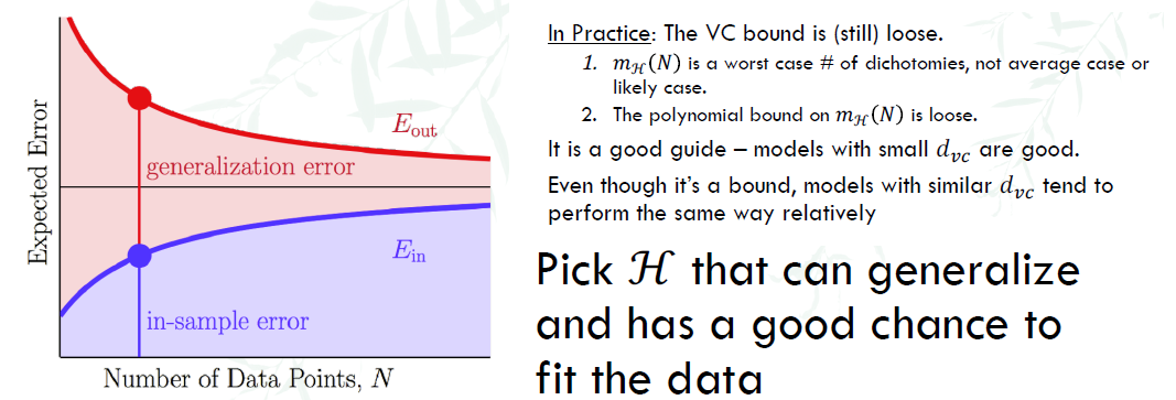
With probability $\geq 1-\delta$, $E_{out}-E_{in} \leq \Omega$ because normally $E_{in} < E_{out}$, we call it generalization error.
$E_{out} \leq E_{in} + \Omega$
With bigger hypothesis set, $E_{in}$ goes down but $\Omega$ goes up. (Worse generalization)

VC Analysis

VC analysis is used to quantify the tradeoff between approximation and generalization. (refer to [Bias and Variance]/BlogSomething2020/posts/cs3244-chap7.html) for more information)

vc graph