Regularization and Validation

Song Jiaming | 18 Nov 2017

This article is a summary note for CS3244 week 8 content. The lecture notes of this course used Caltech’s notes as reference.

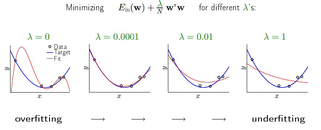
1. Regularization

It constrains the model so that we cannot fit the noise
regularization

Let’s consider the polynomial model:
poly

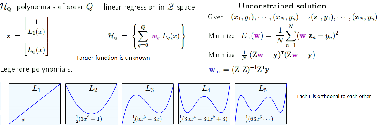
Constraining the weights

Hard constraint: $H_{2}$ is constrained version of $H_{10}$ with $w_{q}=0$ for q > 2
Soft-order constraint: $\sum\limits_{q=0}^{Q} w_{q}^{2} \leq C$
- We still have to min $\frac{1}{N} (Zw-y)^{T}(Zw-y)$
- But cannot choose w freely: subject to $w^{T}w \leq C$
- Solution is called $w_{reg}$ instead of $w_{lin}$ now.

Solving for $w_{reg}$ w_reg

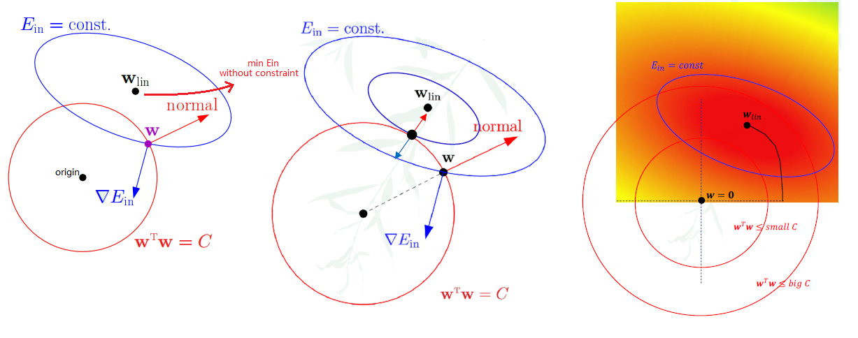
Since we have to choose points within the red circle, the intuitive way is to choose points at the boundary, if we choose w as shown in the first figure in the picture above.
The gradient to the $E_{in}$ eclipse at w is $\triangledown E_{in}$, which is orthogonal to the tangent.
The gradient to the constraint is exactly the direction of vector w.
w is not the minimum, as there is component along the tangent
w achieves minimum when normal and $\triangledown E_{in}$ is at exactly opposite direction
- $\triangledown E_{in} \propto -w_{reg} = -2\frac{\lambda}{N}w_{reg}$ (Constant of proportionality chosen for convenience)
- $\triangledown E_{in} + -2\frac{\lambda}{N}w_{reg} = 0$ which is a solution to $\min \, E_{in}(w) + \frac{\lambda}{N}w^{T}w$
  - when C ↑ , $\lambda$ ↓

Augmented error

\begin{align} \min E_{aug}(w) &= E_{in}(w) + \frac{\lambda}{N} w^{T}w \\ &= \frac{1}{N} (Zw-y)^{T}(Zw-y) + \frac{\lambda}{N} w^{T}{w} \\ &= \frac{1}{N} [(Zw-y)^{T}(Zw-y) + \lambda w^{T}{w}] \end{align}

Corresponding to $\min E_{in}(w)$ subject to $w^{T}w \leq C$ (VC formulation)

The solution to (3) can be obtained by taking derivatives.

$\triangledown E_{aug}(w) = 0 \implies Z^{T}(Zw-y)+\lambda w = 0$
$w_{reg} = (Z^{T}Z + \lambda I)^{-1}Z^{T}y$ (with regularization)
as opposed to $w_{lin} = (Z^{T}Z)^{-1}Z^{T}y$ (without regularization)

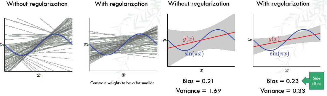
The result
reg

Weight 'decay'
$\min E_{in}(w) + \frac{\lambda}{N}w^{T}w$ is called the weight decay.

Let’s say we use gradient descent: w(t+1) = w(t)- η ∇$E_{in}$(w(t)) - 2 η $\frac{\lambda}{N}$ w(t)
= w(t)(1-2η $\frac{\lambda}{N}$)- η ∇$E_{in}$(w(t)) (shrink the weight first, then move to the suggested direction)
Applies in the neural network: $w^{T}w = \sum\limits_{l=1}^{L}\sum\limits_{i=0}^{d^{l-1}}\sum\limits_{j=1}^{d^{l}}(w_{ij}^{l})^{2}$

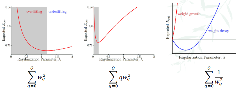
Variations of weight decay

Emphasis of certain weights: $\sum\limits_{q=0}^{Q} \gamma_{q}w_{q}^{2}$
- $\gamma_{q} = 2^{q}$: the regularizer is giving huge emphasis on higher order terms, trying to find as much as possible a low-order fit
- $\gamma_{q} = 2^{-q}$: try to find a high-order fit
- In neural networks: different layers get different $\gamma$
Tikhonov regularizer: $w^{T}\Gamma^{T}\Gamma w$

Weight growth
We constain the weights to be large - bad!

gives λ = 0 the optimal case ⇒ kills the regularization

Weight decay

Practical rule to choose a regularizer

stohastic noise is `high-frequeny’
deterministic noise is also non-smooth
⇒ constrain learning towards smoother hypotheses
- smaller weights correspond to smoother hypothesis

General form of augmented error

The regularizer Ω = Ω(h)
we minimize $E_{aug}(h) = E_{in}(h) +\frac{\lambda}{N}\Omega(h)$
- We have seen $E_{out}(h) \leq E_{in}(h) + \Omega(N,H,\sigma)$ from VC analysis
- $E_{aug}$ can be better than $E_{in}$ as a proxy for $E_{out}$
- There is a complementary relationship between regularization and the VC bound:
  - VC bound deals with the complexity of the hypothesis set Ω(𝑁, 𝓗, 𝛿).
  - Regularization concerns the complexity of the particular hypothesis Ω(h)

Choosing a regularizer

The perfect regularizer Ω is the one constrain in the direction of the target function.

It is not matching the f
It harms the overfitting more than it harms the fitting
It harms fitting the noise more than it harms the signal

Guiding principle:

move in the direction of smoother or ‘simpler’ (because the noise is not smooth)
sacrifice a little bias for large improvement on variance
What if a bad Ω is chosen? We still have λ!

Neural-network regularizers

Weight decay: Refer to the figure 1 below, blue line is the activation function of the neurons.
- Blue-line is the soft threshold. If the signal is very small ⇒ almost linear, if the singnal is ver large ⇒ almost binary
Weight elimination: Fewer weights ⇒ smaller VC dimension
- Soft weight elimination: (similar to weight decay) $\Omega(w) = \sum\limits_{i,j,l} \frac{(w_{ij}^{(l)})^{2}}{\beta^{2}+(w_{ij}^{(l)})^{2}}$
  - for very small w, β dominates, Ω becomes something proportional to $w^{2}$, you are doing weight decay. (for small w, it is pushed to 0, eliminated)
  - for very large w, w dominates, Ω becomes close to 1, nothing to do to change the weights

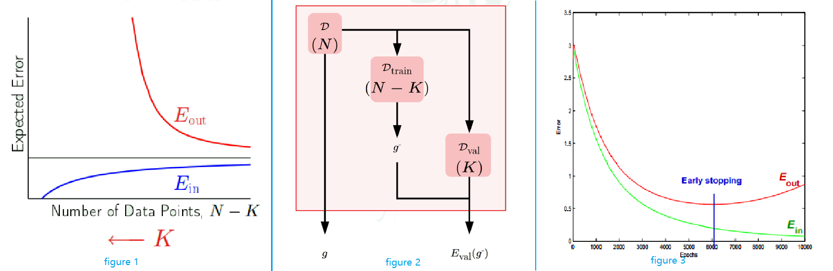
Early Stopping as a regularizer

figure 2 below, stop before you get to the end.
Regularization through the optimiser, instead of through the objective function
Not a porper way of regularization

The optimal λ(figure 3)

Regularizer

2. Validation

$E_{out}(h) = E_{in}(h)$ + overfit penalty

Regularization: estimate the 'overfit penalty' component
Validation estimates $E_{out}$ component

Analyzing the estimate
Out-of-sample points (x,y), the error is e(h(x),y), $E[e(h(x),y)] = E_{out}(h)$, $var[e(h(x),y)] = \sigma^{2}$

Squared error: $(h(x)-y)^{2}$
Binary error: [[$h(x)\not =y$]]

On a validation set (pretend as a out-of-sample set) $(x_{1},y_{1}),…,(x_{K},y_{K})$, the error is $E_{val}(h) = \frac{1}{K} \sum\limits_{k=1}^{K} e(h(x_{k},y_{k})$

$E[E_{val}(h)] = \frac{1}{K} \sum\limits_{k=1}^{K} E[e(h(x_{k},y_{k})] = E_{out}(h)$
$var[E_{val}(h)] = \frac{1}{K^{2}} \sum\limits_{k=1}^{K} var[e(h(x_{k},y_{k})]= \frac{\sigma^{2}}{K}$
$E_{val}(h) = E_{out}(h) \pm O(\frac{1}{\sqrt{K}})$

If K is larger, the estiate is better, however, K is part of the training set

More K for validation ($D_{val}$), less N-K for taining ($D_{train}$)
Samll K ⇒ bad estimate of $E_{out}$
Large K ⇒ Huge real $E_{out}$ (as seen in the figure 1 below)

A way to solve this problem is to put K back into N. (figure 2 below)

D = $D_{train} \cup D_{val}$
The hypothesis trained on D: g
The hypothesis trained on $D_{train}$: $g^{-}$
- Test $g^{-}$ on $D_{val}$ to yield $E_{val}(g^{-})$
- Give g (not $g^{-}$!), $E_{val}(g^{-}$ as result
However, if we have large K, $g^{-}$ is more different than g, so $E_{out}(g^{-})$ will be a bad estimate of the real $E_{out}(g)$
Rule of thumb: $K = \frac{N}{5}$

Validation

Why Validation?

$D_{val}$ is used to make learning choices
Recall figure 3 above, we can stop at lowest $E_{val}$
We can choose the level of regularization to minimize $E_{val}$

What's the difference?

Test set is unbiased, validation set has optimistic bias
2 hypotheses h1 and h2 with $E_{out}(h1) = E_{out}(h2) = 0.5$
Error estimates e1 and e2 uniform on [0, 1]
Pick h ∈ {h1, h2} with e = min(e1,e2)
E[e] < 0.5 ( P(1 of the error < 0.5) = 75% ) ⇒ optimistic bias, but it’s not hurting much.

Model Selection

Using $D_{val}$ more than once. (refer to left figure below)

M models $H_{1}, …, H_{M}$
Use $D_{train}$ to learn $g_{m}^{-}$
Evaluate each $g_{m}^{-}$ using $D_{val}$
Pick the $H_{m}^{\ast}$, which $g_{m^{\ast}}^{-}$ with the smallest $E_{m}^{\ast}$ belongs to. (Bias introduced)

Validation2

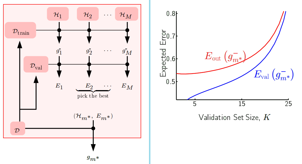
The bias

$E_{val}(g_{m^{\ast}}^{-})$ is a biased estimate of $E_{out}(g_{m^{\ast}}^{-})$
Refer to the right figure above, there are 2 models to choose and affect the curve. (each time I use the model which gives the smallest error)
1. Why the curve goes up? Since the x-axis is the validation size K ⇒ training size N-K is decreasing along x-axis
  - $E_{out}$ curve is the opposite of learning curve
  - $E_{val}$ increases as less training size is used for training
2. Why do the curves get closer together?
  - With more K, estimates get more and more reliable ⇒ close to true error

How much bias?

$D_{val}$ is used for “training” on the finalists model:
- $H_{val} = {g_{1}^{-},…,g_{M}^{-}}$
- By Hoeffding and VC: $E_{out}(g_{m^{\ast}}^{-}) \leq E_{val}(g_{m^{\ast}}^{-}) + O(\sqrt{\frac{\ln M}{K}})$

Data Contamination

Error estimates: $E_{in},E_{out},E_{val}$
Contamination: optimistic (deceptive) bias in estimating $E_{out}$
- Training set: totally contaminated ($E_{in}$ is no estimation to $E_{out}$)
- Validation set: slightly contaminated
- Test set: totally 'clean'

Cross Validation

The dilemma about K

$E_{out}(g) \underset{\text{samll K}}{\approx} E{out}(g^{-}) \underset{\text{large K}}{\approx} E_{val}(g^{-})$
can we have K both small and large?

Leave One Out

N-1 points for training, 1 point for validation
Let all N points take turns to be that 1 validation point

Validation3

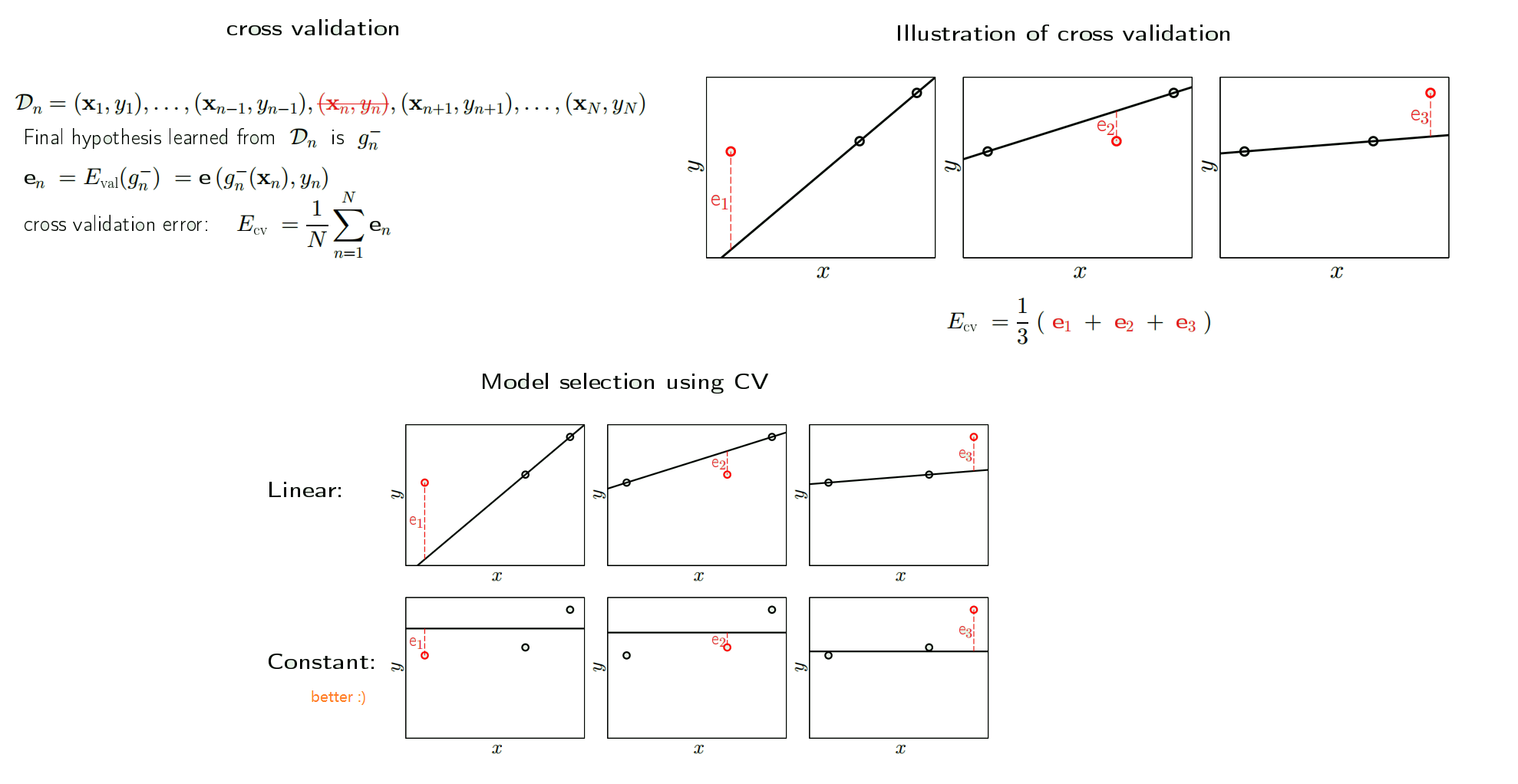
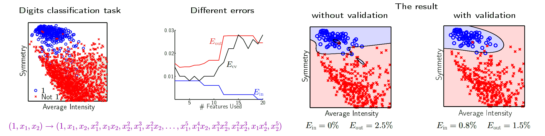
cross validation in action

we try to choose no. of features by $E_{cv}$
From the figure below, we may want to paramters = 6, as it has lower $E_{cv}$
The result is shown in the right, we are better off with validation

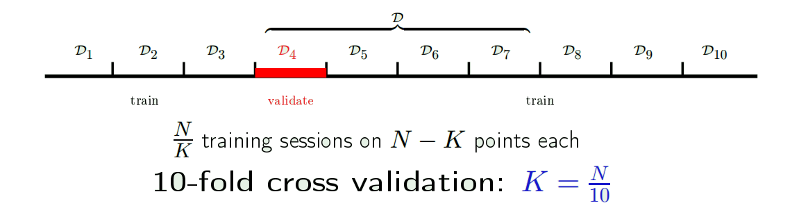
K-fold cross validation
LOOCV can be very expensive for large datasets. You need to train N-1 different $g^{-1}$

Instead, we use K fold cross validation: i.e., K validation set with $\frac{N}{K}$ points each.

Recommend: 10-fold CV

K-fold