Bias and Variance
Song Jiaming | 17 Nov 2017

This article is a summary note for CS3244 week 7 content. The lecture notes of this course used Caltech’s notes as reference.
Approximation-Generalization Tradeoff
Suppose we have a set of hypothesis functions H to approximate f. The ideal case is when H={ f }. However, that’s unlikely to happen.
To be more realistic, we hope our H have a small $E_{out}$, which means H is a good approximation of f for unseen sample (out-of-sample). However, there is a tradeoff:
- Complex H (more hypothesis) → better chance of approximating f
- Simple H (less hypothesis)→ better chance of generalizing unseen sample
Bias-Variance Analysis
We need a way to quantify the above tradeoff. The bias-variance analysis is one way,(VC Analysis is another way) it decomposes $E_{out}$ into 2 components:
- How well H can approximate f overall
- How well we can zoom in on a good h ∈ H
Approach: we apply our H to data and obtain a result, compare this result with the real-valued targets (the true result of data), then use squared error to quantify the difference.
- Start with $E_{out}$:
- Let g ∈ H be a hypothesis, D be a dataset which we trained our g on, x be another dataset which we use g to predict its results.
- Then $E_{out}(g^{(D)}) = E_{x}[ (g^{(D)}(x) - f(x))^{2}]$
- Let g ∈ H be a hypothesis, D be a dataset which we trained our g on, x be another dataset which we use g to predict its results.
- We want to generalizing over all N sets of D, (expectation of D)
- $E_{D}[E_{out}(g^{(D)})] = E_{D}[E_{x}[ (g^{(D)}(x) - f(x))^{2}]]= E_{x}[\bbox[pink]{(E_{D}[(g^{(D)}(x) - f(x))^{2}]} ]$
- To evaluate $E_{D}[(g^{(D)}(x) - f(x))^{2}]$, define average hypothesis $\bar{g}(x) = E_{D}[g^{(D)}(x)]$.
- Imagine we have $D_{1},D_{2},…,D_{k}$, then $\bar{g}(x) \approx \frac{1}{K}\sum\limits_{k=1}^{K} g^{(D)}(x)$
- Then, \begin{align} E_{D}[(g^{(D)}(x) - f(x))^{2}] &= E_{D}[(g^{(D)}(x)- \bar{g}(x) + \bar{g}(x) - f(x))^{2}] \\ &= E_{D}[(\bbox[lightblue]{g^{(D)}(x)- \bar{g}(x)})^{2} + (\bbox[lightGreen]{\bar{g}(x) - f(x)})^{2} + 2(\bbox[lightblue]{g^{(D)}(x)- \bar{g}(x)}\,)(\,\bbox[lightGreen]{\bar{g}(x) - f(x)})] \end{align}
- Since $E_{D}(2(\bbox[lightblue]{g^{(D)}(x)- \bar{g}(x)}\,)(\,\bbox[lightgreen]{\bar{g}(x) - f(x)})) = (E_{D}[g^{(D)}(x)]- \bar{g}(x))(E_{D}[\bar{g}(x) - f(x)]) = (\bar{g}(x)-\bar{g}(x))\cdot C$
- C is a constant
- $\bbox[pink]{E_{D}[(g^{(D)}(x) - f(x))^{2}]} = \bbox[lightblue]{E_{D}[(\bar{g}(x) - f(x))]^{2}} + \bbox[lightgreen]{(\bar{g}(x) - f(x))^{2}}$
- The 1st part highlighted in pink: how far away your hypthesis (on the specific D dataset) is from the true f
- The 2nd part highlighted in blue: how far away is your hypothesis (on the specific D dataset) from the best possible hypothesis you can have (on all Ds)
- This is the var(x)
- Because this measures how far each hypothesis on each D is different from the best hypothesis
- The 3rd part highlighted in green: how far away your best possible hypothesis is from the true f
- This is also the bias(x)
- Because that’s how the best hypothesis set is biased away from f
- Finally, $E_{D}[E_{out}(g^{(D)})] = E_{x}[bias(x)+var(x)]$ = bias + var
Tradeoff
We want to argue that when one of bias or var goes up, the other one goes down.
- Bias = $E_{x}[(\bar{g}(x) - f(x))^{2}]$
- Variance = $E_{x}[E_{D}[(\bar{g}(x) - f(x))]^{2}]$
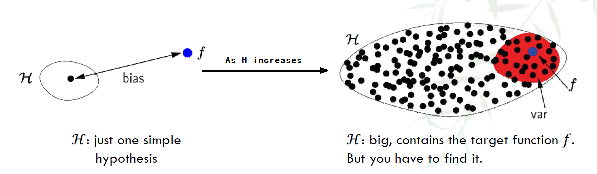
As seen in the figure below:
- When only 1 H exists, the distance is far from f. When there are more H, on average, they are nearer to f than just 1 single H.
- However, for more H, $\bar{g}$ can be at anywhere, where for 1 H, it is the only $\bar{g}$
Thus, As H increases, bias decreases, but variance increases.
Example: Sine targets
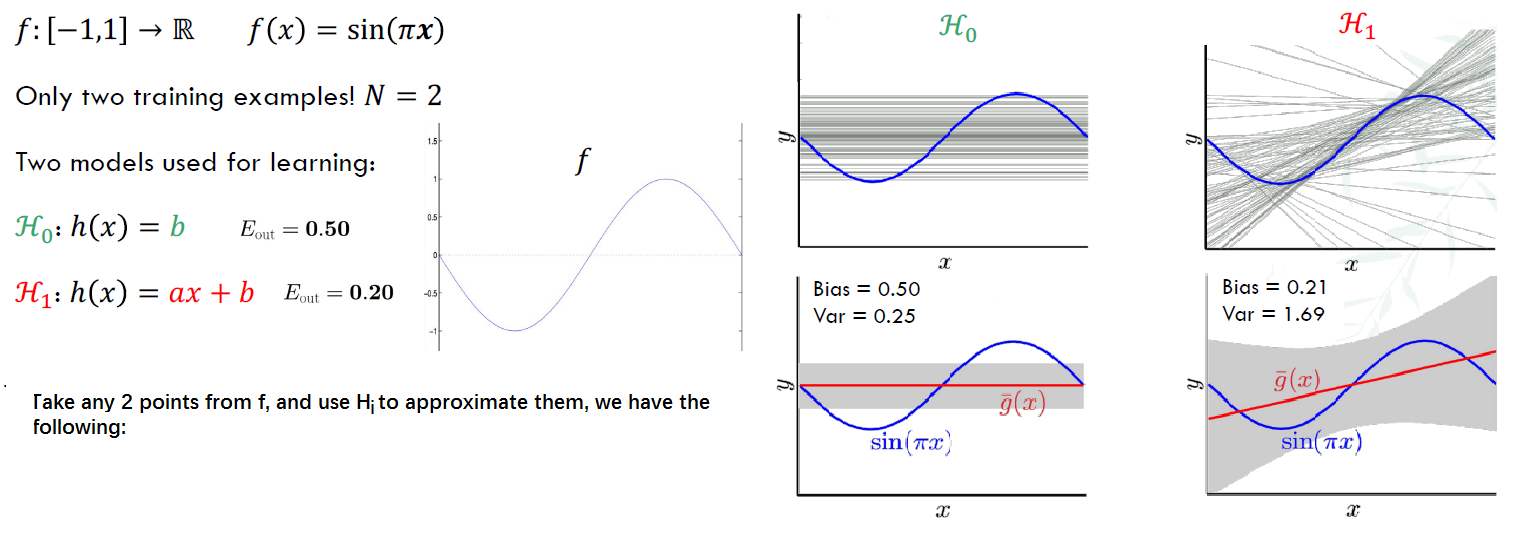 Though $H_{0}$ has high $E_{out}$, it has lower variance, so always match ‘model complexity’ to the data resources, not to the target complexity.
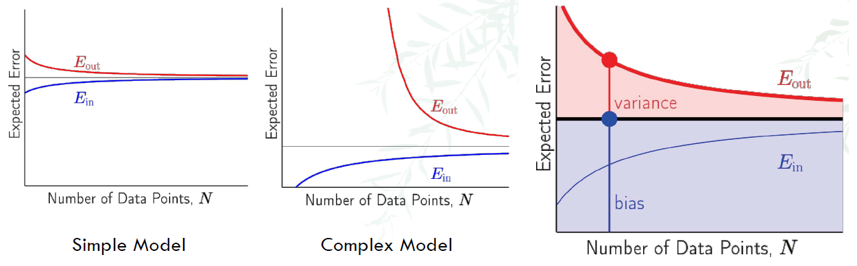
Learning Curve
Given a dataset D of size N, we have:
- Expected out-of-sample error: $E_{D}[E_{out}(g^{(D)})]$
- Expected in-sample error: $E_{D}[E_{in}(g^{(D)})]$
Learning curve is to plot the relationship of how these errors vary with N.
- For simple model, the expected error is higher, but discrepancy between 2 errors is lower
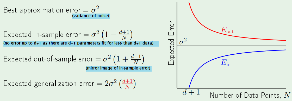
Linear Regression Case
- Noisy target y = $(w^{\ast})^{T}x$ + noise
- Dataset D = ${(x_{1},y_{1}),…(x_{N},y_{N})}$
- Linear regression solution: $w = (X^{T}X)^{-1}X^{T}y$
- In-sample error vector = Xw - y
- ‘Out-of-sample’:
- Generate another target y’ = $(w^{\ast})^{T}x$ + noise’
- Error vector = Xw - y’
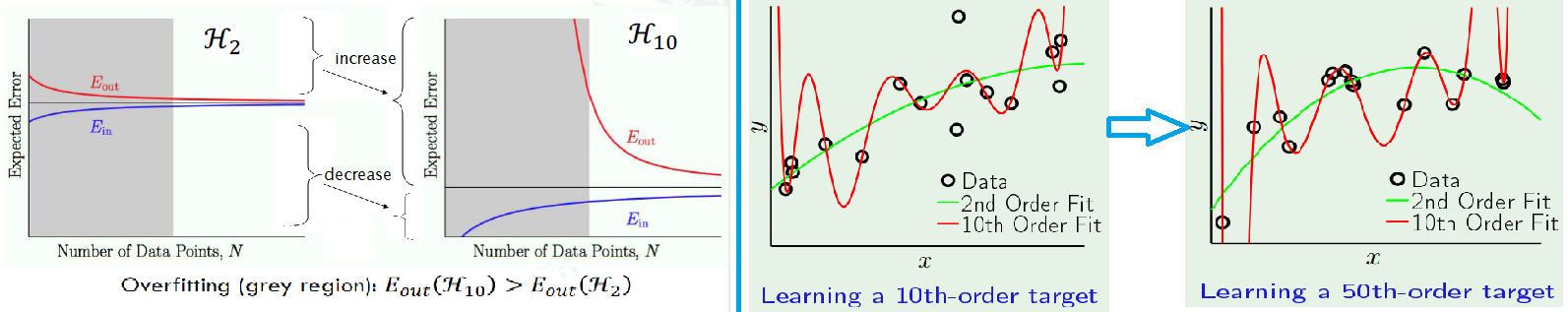
Overfitting
Illustration
Suppose we have 5 data points,
- A simple target function does not fit them perfectly, there must be noise
- A 4th-order polynomial function fit them perfectly, $E_{in}=0$ but $E_{out}$ is huge ⇒ overfitting
- Reason: if 3rd order polynomial is used, $E_{in}$ won’t be 0, but $E_{out}$ will be reduced. So overfitting happens at 4th order, not 3rd order.
Overfitting: fitting the data more than is warranted. (When $E_{in}$ goes down, $E_{out}$ goes up.) It is fitting the noise, it assume noise as a pattern in your sample, which is of course not the case in out-of-sample
Case Study
- We first create dataset by using the 2 polynomials.
- Then, choose another 2 functions,2nd order and 10th order to fit the datasets in the left figure.
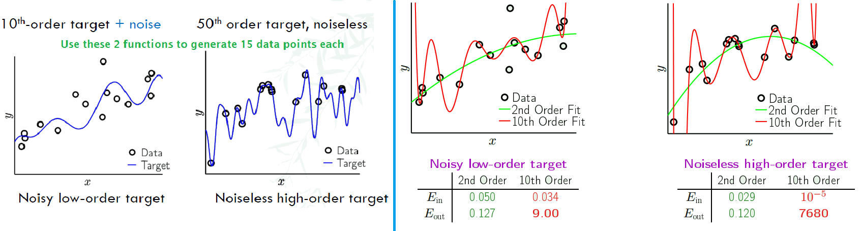
Irony of the 2 learners: O (overfitting) and R (restricted)
We only tell the 2 learners that the target function f is a 10th-order polynomial, and you have to find it by the 15 points given
- O: why not just choose 10th order, $H_{10}$
- R: Only 15 points? I will just choose $H_{2}$ and pray for luck
- So when is $H_{2}$ better, when is $H_{10}$ better?
- Even when there’s no noise, irony(overfitting) still occurs
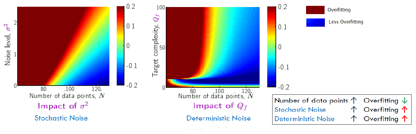
The role of Noise
A detailed experiement
Impact of noise lever and target complexity: $y = f(x) + \epsilon(x) = \bbox[pink]{\sum\limits_{q=0}^{Q_{f}} \alpha_{q} x^{q} }+ \epsilon(x)$
- $\epsilon(x) = \sigma^{2}$, the noise
- $Q_{f}$: Order of the polynomial f, implies the target complexity
- The pink part is the polynomial equation up to degree $Q_{f}$.
- and it’s normalised. (From one degree to another, they are orthogonormal to each other.)
- Dataset size: N
Measure Overfitting:
- still using 2nd-order $g_{2}\in H_{0}$ and 10th order $g_{10}\in H_{10}$
- Overfit measure: $E_{out}(g_{10})- E_{out}(g_{2})$ =
- Positive: More complex one has worse out-of-sample error ⇒ overfitting
- Negative: More complex one did better ⇒ not overfitting
- 0: they are the same
Running 10 millions iterations for the whole process, including:
- Generate a target
- Generate a dataset
- fit both function
- look at the overfit measure
Then we obtain:
| Compare | Stochastic Noise | Deterministic Noise |
|---|---|---|
| Description | Fluctuations/measurement errors we cannot capture | The part of f we lack of capacity to capture |
| formula | $y_{n} = f(x)$ + stochastic | $y_{n} = h^{\ast}(x)$+ deterministic |
| Change H | Remain the same for different hypothesis set | Depends on your hypothesis set |
| Re-fit the same x | Changes | Stay the same |
Noise and Bias-Variance
Recall that $E_{D}[E_{out}(g^{(D)})]$ = bias + var
A noisy target (instead of just f) is $y = f(x) + \epsilon(x)$, where $E[\epsilon(x)] = 0$
A noise term:
\begin{align} E_{D,\epsilon}[ (g^{(D)}(x)-y)^{2} ] &= E_{D,\epsilon}[ (g^{(D)}(x)-f(x) - \epsilon(x))^{2} ] \\ &= E_{D,\epsilon}[ (g^{(D)}(x)- \bar{g}(x) + \bar{g}(x) -f(x) - \epsilon(x))^{2} ] \\&= E_{D,\epsilon}[ \bbox[lightblue]{(g^{(D)}(x)- \bar{g}(x))^{2}} + \bbox[lightgreen]{(\bar{g}(x) -f(x))^{2}} + \bbox[pink]{(\epsilon(x))^{2}} + \text{cross terms} ]\end{align}
- $\bbox[lightblue]{blue}$ part is variance
- $\bbox[lightgreen]{green}$ part is bias, the deterministic noise
- $\bbox[pink]{pink}$ part is $\sigma^{2}$, the stochastic noise.
Two Cures for Overfitting
- Regularization: restrain the model
- Validation: reality check by peeking at the bottom line